Download
1 / 30
300 likes | 491 Vues
Technical Overview of Broadband Powerline (BPL) Communication Systems. Robert G. Olsen School of Electrical Engineering and Computer Science Washington State University Pullman, WA, USA bgolsen@wsu.edu. Presented at University of Idaho October 4, 2006. Injector (2 – 30 MHz).

E N D
Technical Overview of Broadband Powerline (BPL) Communication Systems Robert G. Olsen School of Electrical Engineering and Computer Science Washington State University Pullman, WA, USA bgolsen@wsu.edu Presented at University of Idaho October 4, 2006
Injector (2 – 30 MHz) Photo of a Typical BPL Installation (courtesy B. Cramer EPRI)
The BIG Question Do attenuation, background noise and restricted input power due to emission limits result in the need for financial investment (i.e., for additional equipment, system conditioning, or maintenance) that is incompatible with the requirement that a BPL system be profitable and/or useful to the electric utility? Here, we will look at attenuation and emission issues.
Sources of Channel Attenuation • Ohmic Absorption – generally small • 2. Reflection/Transmission “loss” • (By far the largest component of “loss”) • Reflection/Transmission loss will be examined
HF Transformer Equivalent Circuit At BPL frequencies the transformer presents a highly frequency dependent mismatch to the transmission line
Reflections/Attenuation due to Isolated Junctions Power Line Tap T = 2/3 3.5 dB loss Overhead/Underground Transition Typical Loss = 15 dB
Because the reflections/transmissions from each junction or connected element interact with each other, it is necessary to evaluate the entire system in order to evaluate the system attenuation Z01 Z02 Consider the simple BPL “system” shown next
Attenuation at higher frequencies is very frequency dependent and may exceed 30 dB/km A very messy channel
Broadband Systems for Complex Channels Modulation schemes (such as Orthogonal Frequency Division Multiplexing - OFDM) have been developed for these very complex channels. These schemes spread the signal among numerous carriers over a wide bandwidth. They are designed so that carriers can either be “turned off” or not available due to attenuation without losing the signal. The cost of shutting off carriers to protect licensed operations is a sacrifice in channel capacity.
Emission Issues • Enough power must be used to overcome the • attenuation so that the signal to noise ratio is • sufficiently high for satisfactory communication. • But, larger power causes larger emissions and • these must be controlled so that: • FCC Numerical limits are satisfied • 2. No harmful interference is created. • Balancing attenuation, input power and emissions • (assuming Part 15 as is) results in repeater • spacing of less than 1 km.
Emissions from Balanced Systems Balanced systems (i.e., those with equal and opposite currents on two conductors such as most telephone circuits) emit relatively small fields. This is especially true if the two conductors are closely spaced.
On Meeting Numerical Emission Limits For a two wire power line with 1 meter spacing, the sinusoidal current required to produce a 50 dB V/m equivalent electric field (i.e., the FCC limit in a CISPR QP Rx) at x = 3 meters is 47 A! If Z0 = 550, then the maximum power flowing (without violating the FCC limit) on the transmission line is 1.21 W or –29 dBm! This is not much! It does not take much power to violate the FCC limits. Any unbalance in the currents will increase the fields. Note: Spreading the signal over a wide bandwidth will reduce the measured emissions since CISPR RX bandwidth is only 9 kHz.
Systems that are likely to be Unbalanced • Systems with more than one return path • Systems with significant displacement currents • (i.e., stray capacitance) Fundamental Problem: Since currents are continuous, every current must “return” to its source. The further this return current is from its source current, the greater the emitted fields.
1. Power lines are multiconductor transmission lines as shown below. Current on one phase conductor can return either on the other or on the neutral wire. “Unbalanced” or “common mode” currents that flow on the neutral conductor cause greater emissions
Consider a Typical Excitation System By expanding the voltages and currents into common and differential “modes,” it can be shown that both common and differential modes are excited and that their amplitudes are roughly equal. Tentative conclusion: More complex excitation schemes that excite only differential modes appear to be warranted.
The reality is not so easy. Consider what happens when currents are incident on an unbalanced connected element. A differential mode current will create a common mode current and vice versa
2. Systems with significant displacement currents Source Current Open circuit current
At low frequency, the open circuit current is nearly zero as expected. But not at higher frequencies. Here, displacement currents become important
Decay rate of BPL fields away from a power line Why is this controversial? FCC Section 15.31(f) says: an attenuation factor 40log10(d2/d1) should be used to extrapolate BPL field measurements made at d1 meters to a location d2 meters from the power line. If the field actually decays more slowly than this, measurements made close to the line and extrapolated to 30 meters (the standard distance) will indicate smaller fields than the actual fields measured. Measurements have been reported that support a slower decay rate than suggested by the FCC Do these measurements make sense?
Decay Rate Calculations simplified geometry, assume dpn >> dpp General expression for the magnetic field along x axis I1 + I2 + I3 = 0 Messy, but simplified soon! Most important: x, d’s compared to λ Note: λ = 150 meters at 2 MHz and λ = 10 meters at 30 MHz
Suppose x, (x-dpp), (x+dpn) << λ This is a “low frequency” or “near field” approximation Then the Hankel functions can be approximated using “small argument” approximations. Then A lot simpler! At “large” distances” (i.e., x >> dpp , dpn) the decay is as 1/x2 Id and Ic are the differential and common mode amplitudes
If the common mode current is zero (i.e., Ic = 0) The field decays as 1/x2 as long as x >> dpp(reasonable) This is the decay rate assumed by the FCC in its Part 15 Rules (i.e., 40 log10(d2/d1) or 40 dB/decade). …… But, the common mode is not always zero, the frequency is not always low and near field approximations may not always be allowable.
If the return currents are very far away (i.e., dnp >> x) If, further, the differential mode amplitude is 0, then the fields decay as 1/x (i.e., 20log10(d2/d1) or 20 dB/ decade). Since the reality is probably in between these extreme cases, it is no surprise that measurements indicate decay rates between 20 and 40 dB per decade.
At higher frequencies different approximations can be made and The decay rate in this case might be even smaller than 20 dB/decade The bottom line is that 40 log10(d2/d1) generally does not properly describe the decay rate of BPL fields.
Harmful Interference Clause (b) Operation of an intentional, unintentional, or incidental radiator is subject to the conditions that no harmful interference is caused…. Harmful interference is defined as “any emission radiation or induction which endangers the functioning of a radio navigation service or other safety services or seriously degrades, obstructs or repeatedly interrupts a radio communication service operating in accordance with this chapter.” Harmful interference is still not completely defined!!!
Different “World Views” on Defining Harmful Interference 1. Consider Broadcast TV for example: For Grade B, UHF television service (Channel 2 – 55 MHz) a signal strength contour (i.e., 47 dB μV/m*) is defined that results in satisfactory reception in 50% of the locations, 50% of the time. Interference is deemed negligible if certain D/U (desired to undesired signal) ratios defined by the FCC are exceeded. Note: There is no mention here of the noise floor. Therefore, it may be permissible for an interference signal to exceed the noise floor. * CISPR QP Receiver – 120 kHz Bandwidth
2. ConsiderAmateur Radio* This service is frequency agile and operators often look for parts of the frequency spectrum with “low noise” (includes man-made interference). Measurements at 28 MHz in a quiet area indicate that a noise floor of -10 dBuV/m** is not uncommon. Note: The noise floor defines an acceptable interference level Therefore, it is not acceptable for an interference signal to exceed the noise floor. * Position of the ARRL – not endorsed by the FCC ** CISPR QP Receiver – 9 kHz Bandwidth
World View Comparison Commercial TV (Ch 2 – 55 MHz) Amateur Radio - 28 MHz 47 dBμV/m Grade B signal level BPL @ 30 m D/U guard 29.5 dBμV/m BPL with 20 dB filter 9.5 dBμV/m Noise Floor -10 dBμV/m Acceptable Interference Ranges (Red) BPL rejected by the ARRL since it exceeds the noise floor
The Harmful Interference “Wild Card” Is “harmful interference” any signal that contributes to a measurable increase in the noise floor or should it be defined as signals that exceed a defined amount below a specified protected signal level? At how far from the source must the noise be deemed acceptable (i.e. should points further than 10 meters be protected? 30 meters?) These are questions that only the FCC can answer. And, they will be answered only as the FCC responds to complaints
Where are we now? • BPL has not grown as quickly as its proponents thought. Some utilities have dropped BPL programs. • I know of no one who claims to be making a profit on BPL. • In some cases, there have been no interference complaints, but the business case still has not been satisfied. • Independent economic analysis suggests a difficult business case. • Utilities have many applications that are narrowband. It is possible that narrowband power line communication (i.e., the old PLC) could be used on medium voltage and low voltage systems