Download
1 / 104
1.08k likes | 1.58k Vues
Sampling Theory. Determining the distribution of Sample statistics. Sampling Theory sampling distributions. It is important that we model this and use it to assess accuracy of decisions made from samples. A sample is a subset of the population.

E N D
Sampling Theory Determining the distribution of Sample statistics
Sampling Theorysampling distributions • It is important that we model this and use it to assess accuracy of decisions made from samples. • A sample is a subset of the population. • In many instances it is too costly to collect data from the entire population. Note:It is important to recognize the dissimilarity (variability) we should expect to see in various samples from the same population.
Statistics and Parameters A statistic is a numerical value computed from a sample. Its value may differ for different samples. e.g. sample mean , sample standard deviation s, and sample proportion . A parameteris a numerical value associated with a population. Considered fixed and unchanging. e.g. population mean m, population standard deviation s, and population proportion p.
Observations on a measurement X x1, x2, x3, … , xn taken on individuals (cases) selected at random from a population are random variables prior to their observation. The observations are numerical quantities whose values are determined by the outcome of a random experiment (the choosing of a random sample from the population).
The probability distribution of the observations x1, x2, x3, … , xn is sometimes called the population. This distribution is the smooth histogram of the the variable X for the entire population
the population is unobserved (unless all observations in the population have been observed)
A histogram computed from the observations x1, x2, x3, … , xn Gives an estimate of the population.
A statistic computed from the observations x1, x2, x3, … , xn is also a random variable prior to observation of the sample. A statistic is also a numerical quantity whose value is determined by the outcome of a random experiment (the choosing of a random sample from the population).
The probability distribution of statistic computed from the observations x1, x2, x3, … , xn is sometimes called its sampling distribution. This distribution describes the random behaviour of the statistic
It is important to determine the sampling distribution of a statistic. It will describe its sampling behaviour. The sampling distribution will be used the assess the accuracy of the statistic when used for the purpose of estimation. Sampling theory is the area of Mathematical Statistics that is interested in determining the sampling distribution of various statistics
Many statistics have a normal distribution. This quite often is true if the population is Normal It is also sometimes true if the sample size is reasonably large. (reason – the Central limit theorem, to be mentioned later)
Combining Random Variables Quite often we have two or more random variables X, Y, Z etc We combine these random variables using a mathematical expression. Important question What is the distribution of the new random variable?
Example 1: Suppose that one performs two independent tasks (A and B): X = time to perform task A (normal with mean 25 minutes and standard deviation of 3 minutes.) Y = time to perform task B (normal with mean 15 minutes and std dev 2 minutes.) Let T = X + Y = total time to perform the two tasks What is the distribution of T? What is the probability that the two tasks take more than 45 minutes to perform?
Example 2: Suppose that a student will take three tests in the next three days • Mathematics (X is the score he will receive on this test.) • English Literature (Y is the score he will receive on this test.) • Social Studies (Z is the score he will receive on this test.)
Assume that • X (Mathematics) has a Normal distribution with mean m = 90 and standard deviation s= 3. • Y (English Literature) has a Normal distribution with mean m = 60 and standard deviation s= 10. • Z (Social Studies) has a Normal distribution with mean m = 70 and standard deviation s= 7.
Graphs X (Mathematics) m = 90, s= 3. Z (Social Studies) m = 70 , s= 7. Y (English Literature) m = 60, s= 10.
Suppose that after the tests have been written an overall score, S, will be computed as follows: S (Overall score) = 0.50 X (Mathematics) + 0.30 Y (English Literature) + 0.20 Z (Social Studies) + 10 (Bonus marks) What is the distribution of the overall score, S?
Sums, Differences, Linear Combinations of R.V.’s A linear combination of random variables, X, Y, . . . is a combination of the form: L =aX +bY + … + c (a constant) where a, b, etc. are numbers – positive or negative. Most common:Sum = X +Y Difference = X –Y Others Averages = 1/3X + 1/3Y + 1/3Z Weighted averages = 0.40 X + 0.25 Y + 0.35 Z
Sums, Differences, Linear Combinations of R.V.’s A linear combination of random variables, X, Y, . . . is a combination of the form: L =aX +bY + … + c (a constant) where a, b, etc. are numbers – positive or negative. Most common:Sum = X +Y Difference = X –Y Others Averages = 1/3X + 1/3Y + 1/3Z Weighted averages = 0.40 X + 0.25 Y + 0.35 Z
Means of Linear Combinations If L =aX +bY + …+ c The mean of Lis: Mean(L) =a Mean(X) +b Mean(Y) + … + c mL =a mX +b mY + … + c Most common: Mean( X +Y) = Mean(X) + Mean(Y) Mean(X –Y) = Mean(X) – Mean(Y)
Variances of Linear Combinations If X, Y, . . . are independent random variables and L =aX +bY + …+ c then Variance(L) =a2Variance(X) +b2 Variance(Y) + … Most common: Variance( X +Y) = Variance(X) + Variance(Y) Variance(X –Y) = Variance(X) + Variance(Y) The constant c has no effect on the variance
Example: Suppose that one performs two independent tasks (A and B): X = time to perform task A (normal with mean 25 minutes and standard deviation of 3 minutes.) Y = time to perform task B (normal with mean 15 minutes and std dev 2 minutes.) X and Y independent so T = X + Y = total time is normal with What is the probability that the two tasks take more than 45 minutes to perform?
Example 2: A student will take three tests in the next three days • X (Mathematics) has a Normal distribution with mean m = 90 and standard deviation s= 3. • Y (English Literature) has a Normal distribution with mean m = 60 and standard deviation s= 10. • Z (Social Studies) has a Normal distribution with mean m = 70 and standard deviation s= 7. Overall score, S = 0.50 X (Mathematics) + 0.30 Y (English Literature) + 0.20 Z (Social Studies) + 10 (Bonus marks)
Graphs X (Mathematics) m = 90, s= 3. Z (Social Studies) m = 70 , s= 7. Y (English Literature) m = 60, s= 10.
Determine the distribution of S = 0.50 X + 0.30 Y + 0.20 Z + 10 S has a normal distribution with MeanmS= 0.50 mX + 0.30 mY + 0.20 mZ + 10 = 0.50(90) + 0.30(60) + 0.20(70) + 10 = 45 + 18 + 14 +10 = 87
Graph distribution of S = 0.50 X + 0.30 Y + 0.20 Z + 10
Sampling Theory Determining the distribution of Sample statistics
Sums, Differences, Linear Combinations of R.V.’s A linear combination of random variables, X, Y, . . . is a combination of the form: L =aX +bY + … + c (a constant) where a, b, etc. are numbers – positive or negative. Most common:Sum = X +Y Difference = X –Y Others Averages = 1/3X + 1/3Y + 1/3Z Weighted averages = 0.40 X + 0.25 Y + 0.35 Z
Means of Linear Combinations If L =aX +bY + …+ c The mean of Lis: Mean(L) =a Mean(X) +b Mean(Y) + … + c mL =a mX +b mY + … + c Most common: Mean( X +Y) = Mean(X) + Mean(Y) Mean(X –Y) = Mean(X) – Mean(Y)
Variances of Linear Combinations If X, Y, . . . are independent random variables and L =aX +bY + …+ c then Variance(L) =a2Variance(X) +b2 Variance(Y) + … Most common: Variance( X +Y) = Variance(X) + Variance(Y) Variance(X –Y) = Variance(X) + Variance(Y) The constant c has no effect on the variance
Normality of Linear Combinations If X, Y, . . . are independentNormal random variables and L =aX +bY + …+ c then L is Normal with mean and standard deviation
In particular: X +Y is normal with X –Y is normal with
The distribution of averages (the mean) • Let x1, x2, … , xn denote n independent random variables each coming from the same Normal distribution with mean mand standard deviation s. • Let What is the distribution of
The distribution of averages (the mean) Because the mean is a “linear combination” and
Thus if x1, x2, … , xn denote n independent random variables each coming from the same Normal distribution with mean mand standard deviation s. Then has Normal distribution with
Graphs The probability distribution of the mean The probability distribution of individual observations
Summary • The distribution of the sample mean is Normal. • The distribution of the sample mean has exactly the same mean as the population (m). • The distribution of the sample mean has a smallerstandard deviation then the population. • Averaging tends to decrease variability • An Excel file illustrating the distribution of the sample mean
Example • Suppose we are measuring the cholesterol level of men age 60-65 • This measurement has a Normal distribution with mean m = 220 and standard deviation s= 17. • A sample of n = 10 males age 60-65 are selected and the cholesterol level is measured for those 10 males. • x1, x2, x3, x4, x5, x6, x7, x8, x9, x10, are those 10 measurements Find the probability distribution of Compute the probability that is between 215 and 225
Solution Find the probability distribution of
The Central Limit Theorem The Central Limit Theorem (C.L.T.) states that if n is sufficiently large, the sample means of random samples from any population with mean mand finite standard deviation sare approximately normally distributed with mean mand standard deviation . Technical Note: The mean and standard deviation given in the CLT hold for any sample size; it is only the “approximately normal” shape that requires n to be sufficiently large.
Distribution of x:n = 2 Original Population 30 30 Distribution of x:n = 30 Distribution of x:n = 10 Graphical Illustration of the Central Limit Theorem
Implications of the Central Limit Theorem • The Conclusion that the sampling distribution of the sample mean is Normal, will to true if the sample size is large (>30). (even though the population may be non- normal). • When the population can be assumed to be normal, the sampling distribution of the sample mean is Normal, will to true for any sample size. • Knowing the sampling distribution of the sample mean allows to answer probability questions related to the sample mean.
1) 2) £ £ P ( 45 x 60 ) £ P ( x 47 . 5 ) Solutions:Since the original population is normal, the distribution of the sample mean is also (exactly) normal • 1) m = m = 50 x • 2) s = s = = = n 15 9 15 3 5 x Example Example: Consider a normal population with m = 50 and s = 15. Suppose a sample of size 9 is selected at random. Find:
- - æ ö 45 50 60 50 x - £ £ = £ £ z = ; z P ( 45 x 60 ) P ç ÷ è ø 5 5 s n = - £ £ P ( 1.00 z 2.00) = - = 0 . 8413 0 . 0228 0 . 8185 Example x 45 50 60 - 2.00 1.00 0
- - æ ö x 50 47 . 5 50 x - £ = £ z = ; P ( x 47 . 5 ) P ç ÷ è ø 5 5 s n = £ - P ( z . 5 ) = - = 0 . 5000 0 . 1915 0 . 3085 Example x 47.5 50 0 -0.50
x m = m = s = s = » 109 n 20 50 2 . 83 x x Example Example: A recent report stated that the average cost of a hotel room in Toronto is $109/day. Suppose this figure is correct and that the standard deviation is known to be $20. 1) Find the probability that a sample of 50 hotel rooms selected at random would show a mean cost of $105 or less per day. • 2) Suppose the actual sample mean cost for the sample of 50 hotel rooms is $120/day. Is there any evidence to refute the claim of $109 presented in the report? • Solution: • The shape of the original distribution is unknown, but the sample size, n, is large. The CLT applies. • The distribution of is approximately normal
x - æ ö 105 109 x - z £ = £ z = ; P ( x 105 ) P ç ÷ è ø 2 . 83 s n = £ - P ( z 1 . 41 ) = 0 . 0793 Example 1)