LABVIEW DATA ACQUISITION
LABVIEW DATA ACQUISITION . Spring Semester 2010. Today’s Menu…. Quick review Data Acquisition in terms of analog-to-digital conversion Modes Questions. Analog-to-Digital Converters. Any DAQ device is essentially an A/D Converter


LABVIEW DATA ACQUISITION
E N D
Presentation Transcript
LABVIEW DATA ACQUISITION Spring Semester 2010
Today’s Menu…. • Quick review • Data Acquisition in terms of analog-to-digital conversion • Modes • Questions
Analog-to-Digital Converters • Any DAQ device is essentially an A/D Converter • The performance of a DAQ device is controlled by various factors that affect the digitized signal quality. • These factors will include: • MODE: Differential or RSE • RESOLUTION: (as mentioned during week 4) • SAMPLING RATE • NOISE
MODE • Mode essentially refers to how we wire stuff into the DAQ. • Remember the thermocouple experiment? • In the case of thermocouples we have an instrument (the thermocouple) that consists of two wires (a positive leg and a negative leg). • We need to connect those to the terminals on some DAQ device. • In doing so we had to decide whether it was to be connected in differential mode or reference single-ended mode.
DIFFERENTIAL MODE • The differential connection shown represents an instrument with wires plugged into AI0(+) and AI0(-). • Differential connections are typically used with signals under one volt or when the instrumentation does not meet the criteria for RSE. • In a system wired for differential inputs, each input has its own reference. • Differential inputs are also useful as they eliminate noise problems because any common-mode noise picked up by the wires gets cancelled.
REFERENCE SINGLE ENDED MODE • Note that the instrument below is plugged into ground (GND) and channel AI0(+). • Reference single-ended (RSE) inputs all reference to some common ground. • Typically an experimenter will use this type of connection with relatively high signals (greater than 1V). • In addition to this high voltage the wires coming from the instrument should be relatively short (less than 3 meters) and all of the other input signals to the DAQ share a common ground.
RESOLUTION • Resolution can be thought of as representation. • Resolution is how the analog-to-digital converter (A/D) represents whatever analog signal it receives. • The A/D does this by using a set number of bits. • Assuming some set range (VOLTS) that the signal from the sensor falls into, the A/D breaks this range into a set number of digitized divisions. • The greater the resolution, the more digitized divisions into which the range can be broken. • As resolution increases we are able to detect smaller and smaller changes in voltage.
Quick review from last week: An instrument’s resolving power • Quick Review: • Last week we looked at the resolving power of a data acquisition device. This resolving power represents the “quality” or lowest level of a sensor’s signal that the DAQ device can discern. • This resolution is represented by the “bit level” of the DAQ. • Resolving power of most DAQ boards can range from 12-bit, 14-bit, 16-bit, and upward to 24- and 32-bit systems.
Quick review from last week: An instrument’s resolving power Example: A DAQ board with 16-bit resolution is used to measure a signal with an input range of 0 – 10 VDC. What is the resolving power of this DAQ board? RP = (Input Range) / 2resolution RP = (10V) / 216 = 0.153 mV or 153 microvolts The DAQ board will be able to detect a signal change as small as 153 microvolts.
The DAQ device can only represent the signal it collects on the PC. • A 3-bit analog-to-digital converter is something you may not ever see in a modern laboratory…. • A 3-bit A/D will split the range of whatever signal it receives into 23 or 8 divisions. • The A/D will represent each division as some binary value between 000 and 111. • Each division represents a discrete portion of the overall waveform.
A low number of divisions will show a segmented representation of a given signal. A higher number of divisions shows something that looks closer to the original waveform. Devices with higher resolution (14-bit, 16-bit, etc) give us data that better approximates the original signal
RANGE • Range can be viewed as everything between the minimum and maximum voltage that is being sent to the DAQ device. • The analog-to-digital converter on the DAQ device will need to digitize this input signal. Most DAQ devices offer us the ability to adjust the given range that we want the A/D to convert. • In LabVIEW this can be done through the DAQ Assistant. • Ranges that are seen include: (-10V to +10V), (-20V to +20V), and (0 to +10V). • Ranges in LabVIEW are selectable, so the experimenter can readily change min and max values. • Typically experimenters will adjust the range to take advantage of a given DAQ device’s resolution capability.
GAIN • Suppose that due to time or cost the experimenter in the previous example is simply stuck with the 3-bit DAQ device? • What could an experimenter do in such a case? • One strategy might be to adjust the gain. • When we adjust the gain we are providing amplification to a signal. • gain = multiplier. • Any gain setting changes will occur to the analog signal prior to it being read by the DAQ device. • As we have learned the A/D can only offer a set number of divisions (8, 2048, or 65536) when it digitizes an analog signal. • If a signal comes in low, the A/D may only be able to use some fraction of its divisions to form a representation of the signal. If the signal is increased by a factor of 2 or more then the number of divisions accessed by the A/D increases.
GAIN Example • When the experimenter is collecting the analog signal she notes that it is a waveform that tends to alternate from 0 volts to 5 volts. • The 3-bit device has a range of 0 to 10 volts and can provide 8 discrete divisions to represent any signal. • With the gain setting equivalent to 1 the DAQ device will collect the 0-5 volt signal and digitize it. • However, of the 8-divisions that this 3-bit device may use to digitize the signal, only four will be useable. • The experimenter decides to multiply the gain by 2 and apply this to the analog signal prior to its reaching the DAQ device. • With a gain setting of 2 the analog signal being fed to the DAQ device is now 0 to 10 volts. The A/D will now use all eight of its divisions and the digital representation of the signal appears much more closer to the original. • Thus, adjusting the gain has improved our understanding of the data.
Gain Effect on Resolving Power • In any experiment we seek to get the most understanding out of the response of the system under test. • The smallest detectable change in a signal or the resolving power of a DAQ device can be determined by the following formula: • RP = (Input Range) / (Gain x 2resolution).
Resolving Power Example 1 • Calculate the resolving power of a DAQ board if it has a resolution of 8-bits, 0 – 10 volt input range, and a gain of 1. • RP = (Input Range) / (Gain x 2resolution) • therefore (10V) / (1 x 28) = 39 mV
Resolving Power Example 2 • Calculate the resolving power of a DAQ board if it has a resolution of 8-bits, 0 – 10 volt input range, and a gain of 2. • RP = (Input Range) / (Gain x 2resolution) • therefore (10V) / (2 x 28) = 19 mV
Resolving Power Example 3 • Calculate the resolving power of a DAQ board if it has a resolution of 8-bits, 0 – 10 volt input range, and a gain of 10. • RP = (Input Range) / (Gain x 2resolution) • therefore (10V) / (10 x 28) = 4 mV
DAQ Device Temperature Sensor Pressure Sensor PC Station and Experimenter Experimental Apparatus Sampling Rate • Last week we utilized the LabVIEW DAQ Assistant to communicate with the DAQ device and therefore the sensor it is attached to.
Sampling Rate • In LabVIEW a standard sample is usually 1000 data points. • We decide that the “speed” or frequency that we wish to collect data at will be 1000 Hz. • We can go through the initialization routine with the DAQ Assistant and set up our standard collection parameters in the Timing Settings section of the DAQ Assistant. • This DAQ Assistant has been set-up so that the Acquisition Mode for the device will be to collect N Samples. • We select the value for N as 1000 Samples to Read. • The Rate (Hz) will be a frequency of 1000. • So we have selected our standard data collection settings but what do these parameters actually mean and how will they affect the VI’s overall timing? This is an important question as it pertains to data collection.
Sampling Rate • When we execute the VI with the rate of 1000 Hz and the number of samples set to 1000 data points we may get a result similar to the one in this figure. • In this case we measure the output of a battery pack. The battery pack has a voltage in excess of 6 volts. We run the DAQ frequency at 1000 Hz. • The DAQ collects this information to a buffer. All the data it collects goes to the buffer and is then displayed when the DAQ has finished collecting. • Each data point enters the buffer in the form of an array. Each data point that we collect will be given a specific address within the array. • When it comes time to display this data the first point in will be the first point out. Thus LabVIEW keeps track of the data it collects via the classic first-in/first-out or FIFO method.
Sampling Rate • The VI requires 1 second to collect 1000 data points at 1000 Hz. • This makes sense when we consider the rate. The rate of collection is 1000 Hz or 1000 points per second. • But what if we were measuring some voltage process where we needed to collect data for several seconds? If that were the case then a collection time of 1 second would not be sufficient. • Also, note the overall resolution of our data. We see changes in millivolts. Our total range was 40 volts and the gain was 1. The DAQ device is a 14 bit instrument. Thus our resolution equates to (40V) / (1 x 214) = 2.4 mV. We see that this level of resolution is achieved in the data collected by our VI.
Sampling Rate • Let’s assume we need to take measurements for 4 seconds. • As the rate is set to 1000Hz and we have learned that it takes 1 second to collect 1000 data points. • So let’s adjust the number of samples to 4000. When we run the VI we see the result below. Note that our VI collected data for 4 seconds.
Sampling Rate • You may note that the screen looks remarkably busy! • The VI collected a good deal of information. Perhaps we want less. • Sure, we need to monitor our process for 4 seconds, but perhaps we only need 200 data points. • One way to adjust the amount of information taken in is to change the rate. • If we adjust the rate to 50 Hz and the number of samples to 200. • The results are shown below. There are fewer data points but the range of data is similar to our earlier samples. Also, we are able to collect valuable data on our process in the required 4 seconds.
Sampling Rate • Yet in terms of computer speed 4 seconds is really rather slow. • Can LabVIEW collect data in shorter periods of time? • The answer is yes! • We can do this by adjusting the rate and number of samples collected. • Let’s say we needed to collect information in 1/10th of a second. • We could adjust our rate to 1000 Hz and then collect 100 samples.
Sampling Rate • Clock rate for this DAQ instrument allows us to take samples at a rate up to 48000 Hz. • This is very useful if we have a situation in which we need to record some event very quickly. • If an experiment was conducted where we had to monitor an event that happened in less than 200 micro-seconds LabVIEW could help us. • This could be a controlled detonation like the ignition of a model rocket engine or a chemical reaction in which a precipitate forms in solution. • In this case we would apply the maximum collection rate and opt to collect 10 samples within that interval.
Sampling Rate • How might we go about recording an event over several minutes? • Let’s say we wanted to monitor a robotic arm’s position and needed to capture data for 120 seconds. • In the prior examples we became fairly adept at finding combinations of rates and samples to adjust our sample collection time as well as the quantity of data points collected. • We will set a rate of 1 Hz and request 120 samples be collected. The VI will capture 120 seconds of data. • We could also set the rate to 1000 Hz and 120000 points or 0.5 Hz and 60 points. • It all depends on how many samples we feel we need. • Yet when we go to run our VI for the two minutes that the experiment requires we notice that at around the 10 second mark the DAQ Assistant flashes ominously and this message appears: Our beloved VI has crashed!
Sampling Rate • We noted that the DAQ Assistant made a weird little flash just before our VI crashed. • And so we take a closer look at it. Near the bottom of the menu under the DAQ Assistant we note something we may have overlooked earlier. What, we ask, is this orange terminal labeled timeout? • With further investigation we realize that the DAQ Assistant has a default setting in which it will only collect data for 10 seconds. This is an important discovery because sometimes we need to collect data for longer periods of time! • If you set the timeout to a value of -1 the VI will not shutdown until it has collected all of the data that you have programmed it to collect. • This is done by using the Wiring Tool to connect a constant to timeout. When we run our VI again we get a full two minutes of data.
Sampling Rate • In all of our examples we have collected data at varying rates and sample sizes. • This has been done to illustrate VI timing. When we create a VI we may want it to collect data for a very specific rate of time. • When dealing with measurements it is important also to understand that there are set collection rates that work better than others, and that if we set a rate too low we can lose valuable information. • Next week we will explore what this means and a tool that we can use to assure ourselves that we are seeing all of the data that is relevant to our experiment.
NOISE • Noise is anything that might interfere with the proper collection of a signal. • Noise can sometimes be referred to EMI • Anytime we run a wire we are effectively creating an antenna. • This “antenna” can pick up aberrant noise. • There are various strategies for reducing noise, including adding a resistor to a line to reduce bias on a multiplexer, RF clamps, and shielding.