Algorithmic Models for Sensor Networks
170 likes | 301 Vues
This paper discusses the development of algorithms to analyze and ensure the correctness of models for Wireless Sensor Networks (WSNs). It emphasizes the trade-off between simplifying models for tractable analysis and maintaining important network characteristics. Various representations, including graph and geometric, are explored, as well as different connectivity models like UDG and QDG. The paper delves into factors affecting network performance such as node interference, transmission ranges, and node distribution. It concludes that no single model suffices and advocates for conservative modeling approaches for accuracy.

Algorithmic Models for Sensor Networks
E N D
Presentation Transcript
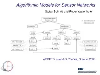
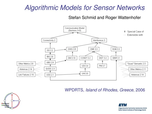
Algorithmic Models for Sensor Networks Schmid, Wattenhofer IPDPS’06
Models and Sensor Networks • To develop algorithms and mathematically prove their correctness, simplifying models are needed for WSN’s. • Balance between simplifying the model in order to keep the analysis tractable and neglecting important properties of the nw • Common representations are as a graph, geometric representation.
Connectivity Models • Given a set of nodes, which nodes can recv the transmission of a given node • Is u adjacent to v ? • Typically symmetric. • Classic model UDG • Transmission range normalized to 1
UDG • Idealistic since real radios are not omni directional and even small obstacles affect connectivity • Proposed General Graph
Connectivity models (contd.) • Too pessimistic! • Something between the 2 extremes. • QDG with ρ=1 is a UDG
UDG to QUDG • Many algorithms can be transformed from UDG to QUDG at a cost of 1/ρ2 • This ok for ρ=0.5 (4) • But for ρ=0.1, much worse (100) • Still does not translate nicely to obstacles like walls – eg. All nodes on one side of the wall can talk to each other but not the opposite side
Extending the dimension • 2d • Nodes in 2d Euclidean plane form a doubling metric • General graph does not
Additional variations • Antennas variations besides omni-directional • Link failures – model probabilistically
Interference • Important for lower layer protocols • Most popular: SINR Signal to Noise Interference Ratio • Does not specify power. 3 ways:
Interference • The SINR model is very complicated • A lot of far away transmissions sum up as noise to a sender-receiver pair • ONE is popular. UDG with one – UDI shown next
Algorithms • Global – can operate on entire network • Distributed – a node has information about only its own state. Messages need to be exchanged to learn more about the nw. All nodes run their own algorithm • Localized – Special case of distributed. Limited to k. A node can retard its right to communicate i.e. some causality
Other assumptions • MAC – ideal vs. interference (adversary) • Random node distribution – uniform distribution in 2d plane. Also Poisson • Worst-case node distribution – completely arbitrary • Node id’s – again worst, random. Range can limit also
Other assumptions • Location info: absolute or relative to other nodes. • Sleep time energy consumption • Lifetime definitions.
Conclusion • No one model • Emphasized that for correctness, the more pessimistic or conservative models should be used • Broad overview provided.