Graphical Models, Distributed Fusion, and Sensor Networks
470 likes | 623 Vues
Graphical Models, Distributed Fusion, and Sensor Networks. Alan S. Willsky February 2006. One Group’s Journey. The launch: Collaboration with Albert Benveniste and Michelle Basseville

Graphical Models, Distributed Fusion, and Sensor Networks
E N D
Presentation Transcript
Graphical Models, Distributed Fusion, and Sensor Networks Alan S. Willsky February 2006
One Group’s Journey • The launch: Collaboration with Albert Benveniste and Michelle Basseville • Initial question: what are wavelets really good for (in terms that a card-carrying statistical signal processor would like) • What does optimal inference mean and look like for multiresolution models (whatever they are) • The answer (at least our answer): Stochastic models defined on multiresolution trees
MR tree models as a cash cow • MR models on trees admit really fast and scalable algorithms that involve propagation of statistics up and down (more generally throughout the tree) • Generalization of Levinson • Generalization of Kalman filters and RTS smoothers • Calculation of likelihoods • …
Milking that cow for all it’s worth • Theory • Old control theorists never die: Riccati equations, MR system theory, etc. • MR models of Markov processes and fields • Stochastic realization theory and “internal models” • MR internal wavelet representations • New results on max-entropy covariance extension—with some first bits of graph theory
Keep on milking… • Applications • Computer vision/image processing • Motion estimation in image sequences • Image restoration and reconstruction • Geophysics • Oceanography • Groundwater hydrology • Helioseismology (???) • Other fields I don’t understand and probably can’t spell
Sadly, cows can’t fly (no matter how hard they flap their ears) • The dark side of trees is the same as the bright side: No loops • Try #1: Pretend the problem isn’t there • If the real objectives are at coarse scales, then fine-scale artifacts may not matter • Try #2: Beat the dealer • Cheating: Averaging multiple trees • Theoretically precise cheating: Overlapping trees • Try #3: Partial (and later, abject) surrender • Put the &#%!*@# loops in!! • Now we’re playing on the same field (sort of) as AI graphical model-niks and statistical physicists
Graphical Models 101 • G = (V, E) = a graph • V = Set of vertices • E VV = Set of edges • C = Set of cliques • Markovianity on G(Hammersley-Clifford)
Algorithms that do this on trees • Message-passing algorithms for “estimation” (marginal computation) • Two-sweep algorithms (leaves-root-leaves) • For linear/Gaussian models, these are the generalizations of Kalman filters and smoothers • Belief propagation, sum-product algorithm • Non-directional (no root; all nodes are equal) • Lots of freedom in message scheduling • Message-passing algorithms for “optimization” (MAP estimation) • Two sweep: Generalization of Viterbi/dynamic programming • Max-product algorithm
What do people do when there are loops? • One well-oiled approach • Belief propagation (and max-product) are algorithms whose local form is well defined for any graph • So why not just use these algorithms? • Well-recognized limitations • The algorithm fuses information based on invalid assumptions of conditional independence • Think Chicken Little, rumor propagation,… • Do these algorithms converge? • If so, what do they converge to?
Example: Gaussian fields • x = (0-mean) Gaussian field on G • Inverse covariance, P-1, is G-sparse • y = Cx + v(indep. measurements at vertices) • If the graph has loops • Gaussian elim. (RTS smoothing) leads to “fill” • Belief propagation (if it converges) yields correct estimates but wrong covariances • Leads to the idea of iterative algorithms using Embedded Trees (or other tractable structures)
Near trees can help cows at least to hover… Tree Exact Covariance Tree Covariance Near-Tree Covariance Near-Tree
Something else we’ve been doing: Tree-reparameterization • For any embedded acyclic structure:
So what does any of this have to do with distributed fusion and sensor networks? • Well, we are talking about passing messages and fusing information • But there are special issues in sensor networks that add some twists and require some thought • And that also lead to new results for graphical models more generally
A first example: Sensor Localization and Calibration • Variables at each node can include • Node location, orientation, time offset • Sources of information • Priors on variables (single-node potentials) • Time of arrival (1-way or 2-way), bearing, and absence of signal • These enter as edge potentials • Modeling absence of signals may be needed for well-posedness, but it also leads to denser graphs
Even this problem raises new challenges • BP algorithms require sending messages that are likelihood functions or prob. distributions • That’s fine if the variables are discrete or if we are dealing with linear-Gaussian problems • More generally very little was available in the literature (other than brute-force discretization) • Our approach: Nonparametric Belief Propagation (NBP)
Nonparametric Inference for General Graphs Belief Propagation Particle Filters • General graphs • Discrete or Gaussian • Markov chains • General potentials Nonparametric BP • General graphs • General potentials Problem: What is the product of two collections of particles?
Nonparametric BP Stochastic update of kernel based messages: I. Message Product: Draw samples of from the product of all incoming messages and the local observation potential II. Message Propagation: Draw samples of from the compatibility function, , fixing to the values sampled in step I Samples form new kernel density estimate of outgoing message (determine new kernel bandwidths)
NBP particle generation • Dealing with the explosion of terms in products • How do we sample from the product without explicitly constructing it? • The key issue is solving the label sampling problem (which kernel) • Solutions that have been developed involve • Multiresolution Gibbs sampling using KD-trees • Importance sampling
Setting up graphical models • Different cases • Cases in which we know which targets are seen by which sets of sensors • Cases in which we aren’t sure how many or which targets fall into regions covered by specific subsets of sensors • Constructing graphical models that are as sensor-centric as possible • Very different from centralized processing • Each sensor is a node in the graph (variable = assigning measurements to targets or regions) • Introduce region and target nodes only as needed in order to simplify message passing (pairwise cliques)
Communications-sensitive message-passing • Objective: • Provide each node with computationally simple (and completely local) mechanism to decide if sending a message is worth it • Need to adapt the algorithm in a simple way so that each node has a mechanism for updating its beliefs when it doesn’t receive a full set of messages • Simple rule: • Don’t send a message if the K-L divergence from the previous message falls below a threshold • If a node doesn’t receive a message, use the last one sent (which requires a bit of memory: to save the last one sent)
Illustrating comms-sensitive message-passing dynamics Organized network data association Self-organization with region-based representation
Incorporating time, uncertain organization, and beating the dealer • Add nodes that allow us to separate target dynamics from discrete data associations • Perform explicit data association within each frame (using evidence from other frames) • Stitch across time through temporal dynamics
How different are BP messages? • Message “error” as ratio (or, difference of log-messages) • One (scalar) measure • Dynamic range • Equivalent log-form
Why dynamic range? • Satisfies sub-additivity condition • Message errors contract under edge potential strength/mixing condition
Results using this measure • Best known convergence results for loopy BP • Result also provides result on relative locations of multiple fixed points • Bounds and stochastic approximations for effects of (possibly intentional) message errors
Experiments • Stronger potentials • Loopy BP not guaranteed to converge • Estimate may still be useful • Relatively weak potential functions • Loopy BP guaranteed to converge • Bound and estimate behave similarly
Communicating particle sets • Problem: transmit Niid samples • Sequence of samples: • Expected cost is ¼ N*R*H(p) • H(p) = differential entropy • R = resolution of samples • Set of samples • Invariant to reordering • We can reorder to reduce the transmission cost • Entropy reduced for any deterministic order • In 1-D, “sorted” order • In > 1-D, can be harder, but…
Trading off error vs communications • KD-trees • Tree-structure successively divides point sets • Typically along some cardinal dimension • Cache statistics of subsets for fast computation • Example: cache means and covariances • Can also be used for approximation… • Any cut through the tree is a density estimate • Easy to optimize over possible cuts • Communications cost • Upper bound on error (KL, max-log, etc)
Examples – Sensor localization • Many inter-related aspects • Message schedule • Outward “tree-like” pass • Typical “parallel” schedule • # of iterations (messages) • Typically require very few (1-3) • Could replace by msg stopping criterion • Message approximation / bit budget • Most messages (eventually) “simple” • unimodal, near-Gaussian • Early messages & poorly localized sensors • May require more bits / components…
How can we take objectives of other nodes into account? • Rapprochement of two lines of inquiry • Decentralized detection • Message passing algorithms for graphical models • We’re just starting, but what we now know: • When there are communications constraints and both local and global objectives, optimal design requires the sensing nodes to organize • This organization in essence specifies a protocol for generating and interpreting messages • Avoiding the traps of optimality for decentralized detection for complex networks requires careful thought
A tractable and instructive case • Directed set of sensing/decision nodes • Each node has its local measurements • Each node receives one or more bits of information from its “parents” and sends one or more bits to its “children” • Overall cost is a sum of costs incurred by each node based on the bits it generates and the value of the state of the phenomenon being measured • Each node has a local model of the part of the underlying phenomenon that it observes and for which it is responsible • Simplest case: the phenomenon being measured has graph structure compatible with that of the sensing nodes
Person-by-person optimal solution • Iterative optimization of local decision rules: A message-passing algorithm! • Each local optimization step requires • A pdf for the bits received from parents (based on the current decision rules at ancestor nodes) • A cost-to-go summarizing the impact of different decisions on offspring nodes based on their current decision rules
What happens with more general networks? • Basic answer: We’ll let you know • What we do know: • Choosing decision “rules” corresponds to specifying a graphical model consisting of • The underlying phenomenon • The sensor network (the part of the model we get to play with) • The cost • For this reason • There are nontrivial issues in specifying globally compatible decision “rules” • Optimization (and for that matter cost evaluation) is intractable, for exactly the same reasons as inference for graphical models
Alternate approach to approximate inference: Recursive Cavity Models
Walk-sums, BP, and new algorithmic structures • Focus (for now) on linear-Gaussian models • For simplicity normalize variables so that P-1 = I – R • R has zero diagonal • Non-zero off-diagonal elements correspond to edges in the graph • Values equal to partial correlation coefficients
Walk-sums, Part II • For “walk-summable” models P = (I – R)-1 = I+R+R2+… • For any element of P, this sum corresponds to so-called “walk-sums” • Sums of products of elements of R corresponding to walks from one node to another • BP computes strict subseries of the walk sums for the diagonal elements of P, which leads to • The tightest known conditions for BP mean and covariance convergence (and characterization of the really strange behavior (negative variances) that can occur otherwise) • A variety of emerging new algorithms that can do better • The idea of exploiting local memory for better distributed fusion
Gaussian Walk-Sums and BP • Inference = Walk-Sums on a weighted graph G • Edge weights are partial correlations. • Walk-Summable if spectral radius < 1. • The weight of a walk is product of edge weights. • Correlations = sum over all walks from u to v. • Variances = sum over all self-return walks at v. • Means = re-weighted walk-sum over all walks to v. • BP on Trees = recursive walk-sum calculation • Loopy BP = BP on “computation tree” of G • LBP converges in walk-summable models • Captures only “back-tracking” self-return walks • Captures (1,2,3,2,1). • Omits (1,2,3,1)
Walk-sums, Part III • Dynamic systems interpretation and questions: • BP performs this computation via a distributed algorithm with local dynamics at each node with minimal memory • Remember the most recent set of messages • Full walk-sums are realizable with local dynamics only of very high dimension in general • Dimensions that grow with graph size • There are many algorithms with increased memory that calculate larger subseries • E.g., include one more path • State or “node” augmentation (e.g., Kikuchi, GBP) • What are the subseries that are realizable with state dimensions that don’t depend on graph size?
So where are we going? - I • Graphical models • New classes of algorithms • RCM++ • Algorithms based on walk-sum interpretations and realization theory for graphical computations • Theoretical analysis and performance guarantees • Model estimation and approximation • Learning graphical structure • From data • From more complex models • An array of applications • “Bag of parts” models for object recognition (and maybestructural biology) • Fast surface reconstruction and visualization • …
So where are we going? - III • Information science in the large • These problems are not problems in signal processing, computing, information theory • They are problems in all of these fields • And we’ve just scratched the surface • Why should the graph of the phenomenon be the same as the sensing/communication network? • What if we send more complex messages with protocol bits (e.g. to overcome BP over-counting) • What if nodes develop protocols to request messages • In this case “no news” IS news…