Covariance Vs Correlation Matrix
Covariance Vs Correlation Matrix Use covariance or correlation matrix? If variables are not in the same units Use Correlations Dim(V) =Dim(R) = pxp and if p is large Dimension reduction. Sample Correlation Matrix. Scatterplot Matrix. Linear Algebra

Covariance Vs Correlation Matrix
E N D
Presentation Transcript
Covariance Vs Correlation Matrix • Use covariance or correlation matrix? If variables are not in the same units Use Correlations • Dim(V) =Dim(R) = pxp and if p is large Dimension reduction.
Sample Correlation Matrix Scatterplot Matrix
Linear Algebra Linear algebra is useful to write computations in a convenient way. Singular Value Decomposition: X = U D V’ nxp nxp pxp pxp X centered =>S = V D2 V’ pxp pxp pxp pxp Principal Components(PC): Columns of V. Eigenvalues (Variance of PC’s): Diagonal elements of D2 Correlation Matrix: Subtract mean of rows of X and divide by standard deviation and calculate the covariance If p > n then SVD: X’ = U D V’ and S = U D2 U’ pxn pxn nxn nxn
4 10 2 5 0 PC2 -2 0 -4 -5 -5 0 5 10 -10 -5 0 5 PC1 PC1 (a) Cells are the observations Genes are the variables (b) Genes are the observations Cells are the variables Principal components of 100 genes. PC2 Vs PC1.
Dimension reduction: • Choosing the number of PC’s • k components explain some percentage of the variance: 70%,80%. • k eigenvalues are greater than the average (1) • Scree plot: Graph the eigenvalues and look for the last sharp decline and choose k as the number of points above the cut off. • Test the null hypothesis that the last m eigenvalues are equal (0) • The same idea can be applied to factor analysis.
The top 5 eigenvalues explain 81% of variability. • Five eigenvalues greater than the average 2.5% • Scree Plot • Test statistic is 4 significant for 6 and highly significant for 2. average
f.pca = function (tr) { trb <- tr - (mu <- f.rmean(tr)) trb.svd <- svd(trb) scores <- t(trb) %*% trb.svd$u dimnames(scores)[[2]]<- paste("PC",1:ncol(scores),sep= "") list(sdev = trb.svd$d/sqrt(ncol(tr)), loadings = trb.svd$u, center = mu,scale=rep(1, length(mu)),n.obs = ncol(tr), scores = scores)}
Biplots • Graphical display of X in which two sets of markers are plotted. • One set of markers a1,…,aG represents the rows of X • The other set of markers, b1,…, bp, represents the columns of X. • For example: X = UDV’X2 = U2D2V2’ • A = U2D2a and B=V2D2b, a+b=1 so X2=AB’ • The biplot is the graph of A and B together in the same graph.
Biplot of the first two principal components. Biplot of the first two Factors (rotated).
Ggobi display finding four clusters of tumors using the PP index on the set of 63 cases. The main panel shows the two dimensional projection selected by the PP index with the four clusters in different colors and glyphs. The top left panel shows the main controls and the left bottom panel displays the controls and the graph of the PP index that is been optimized. The graph shows the index value for a sequence of projection ending at the current one.
Generalized Linear Models 1. There is a response y and predictors x1,…, xp. 2. y depends on the x’s through a l.c. h= b1x1+…+ bnxp. 3. The density of y is f(yi,qi,j) = exp[Ai{yi qi- g(qi)}/ j + t(yi ,j/Ai) ] 4. Mean(y)=m =m(h), h=m-1(m) = l(m) : link function