Download
1 / 50
510 likes | 725 Vues
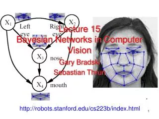
Lecture 15 Bayesian Networks in Computer Vision. Gary Bradski Sebastian Thrun. *. http://robots.stanford.edu/cs223b/index.html. What is a Bayesian Network?. It’s a Factored Joint Distribution and/or Causal Diagram. P(W). (random) variables.

E N D
Lecture 15Bayesian Networks in Computer Vision Gary Bradski Sebastian Thrun * http://robots.stanford.edu/cs223b/index.html
What is a Bayesian Network? It’s a Factored Joint Distribution and/or Causal Diagram P(W) (random) variables A conditional probability distribution quantifies the effects of the parents on node. The graph is directed and acyclic. causal links dependencies P(A|W) P(C|W) P(R|C,A) P(F|C) A joint distribution, here p(W,C,A,R,R), is everything we can know about the problem, but it grows exponentially, here 25-1=31. Factoring the distribution in a Bayesnet decreases the number of parameters, here from 31 to 11(note probabilities sum to one which decreases the number of parameters to be specified).
Causality and Bayesian Nets • One can also think of Bayesian Networks as a “Circuit Diagram” of Probability Models • The Links indicate causal effect, not direction of information flow. • Just as we can predict effects of changes on the circuit diagram, we can predict consequences of “operating” on our probability model diagram. Diode Mains Capac. Transf. Diode Observed Ammeter Un-Observed Battery
Inference • Once we have a model, we need to make it consistent by “diffusing” the distributions around until they are all consistent with one another. • Central algorithm for this: Belief Propagation
“Causal” message “Diagnostic” message Messages Specifically: 1/a 9 Bayes Law: Belief Propagation Going down arrow, sum out parent Going up arrow, Bayes Law Message * some figures from: Peter Lucas BN lecture course
Diagnostic message against arrow Causal message with arrow Bayes Law: Belief Propagation * some figures from: Peter Lucas BN lecture course
Inference in general graphs • Belief propagation is only guaranteed to be correct for trees • A general graph should be converted to a junction tree, by clustering nodes • Computationally complexity is exponential in size of the resulting clusters (NP-hard)
X1 X1 X1 X3 X2 X3 X3 X2 X2 X5 X4 X5 X5 X4 X4 X6 X6 X6 Junction tree: BN Junction Tree Algorithm for turning a Bayesian Network with loops into a junction tree • “Moralize” the graph by connecting parents • Drop the arrows. • Triangulate (connect nodes if a loop of >3 exists) • Put in intersection variables Graph: (1) (2) (3) X1 X3 X2 X5 X4 X6 Junction Tree: Image from Sam Roweis * Lauritzen 96
Distribute Collect root root root root Global message passing: Two pass • Select one clique as the root • Two pass message passing: first collect evidence, then distribute evidence. Figure from P. Green
Junction Tree Inference Image from Cecil Huang
X1 X3 X4 X2 Stage 1. Stage 2. X1 X3 X4 X2 Global message passing: Parallel, distributed version • All nodes can simultaneously send messages out, if it has received the messages from all its parents • Parallel processing (topology level parallelism).
Details Junction Tree Algorithm
a b {c,d} c {c} d e a b {a,b,c} {c} {c,e} c d e Junction Tree Properties Graph: Moralized, triangular graph: An undirected graph whose vertices (clusters) are sets of variables with three properties: • Singly connected property (only one path) • Potential property (all variables are represented) • Running intersection property (variable in 2 nodes implies that all nodes on the path have the variable) Junction Tree: Collect and Distribute pass necessary for Inference
Junction Tree 1 Image from Sam Roweis
Junction Tree 2 Image from Sam Roweis
Message Passing in Junction Tree • Potential • U, the space of U (subset of the set of all nodes/vertices V) is the Cartesian product of the state sets of the nodes of U • A discrete potential on U is a mapping from U to the non-negative real numbers Ro. • Each clique and seperator in the junction tree has a potential (actually marginalized joint distribution on the nodes in the clique/seperator) • Propagation/message passing between two adjacent cliques C1, C2 (S0 is their seperator) • Marginalize C1’s potential to get new potential for S0 • Update C2’s potential • Update S0’s potential to its new potential
Message Passing General • BayesNet forms a tree • Pearl’s algorithm is Message Passing first out and then back in from a given node • Not a tree (has loops) • Turn loops into cliques until net is a tree, then use Pearl’s algorithm • Cliques turn out to be too big • Exact computation is exponential in size of largest cliques • Use approximation algorithms (many)
From Bayes’ Net to Decision/Influence Network Start out with a causal Bayesian Network. In this case, Possible causes of leaf loss in an apple tree. We want to know what to do about this. We duplicate the network because we are going to Add an intervention: Treating sickness The intervention will cost us, but might help with our utility: Making a profit when we Harvest. Given the cost, we can now infer the optimal Treat/no-treat policy
No fever, no runny nose healthy, don’t treat No fever means, cold less likely => Treat No fever, runny nose => allergy => treat Replicate cold net and add decision and cost/utility nodes Influence Example
Probabilistic graphical models Probabilistic models Graphical models Directed Undirected (Bayesian belief nets) (Markov nets) Alarm network State-space models HMMs Naïve Bayes classifier PCA/ ICA Markov Random Field Boltzmann machine Ising model Max-ent model Log-linear models
Typical forms for the Conditional Probability Distributions (CPDs)at graph nodes • For Discrete-statenodes • Tabular (CPT) • Decision tree • Deterministic CPD • SoftMax(logistic/sigmoid) • Noisy-OR • MLP • SVM? • For Continuous-state nodes • Gaussian • Mixture of Gaussians • Linear Gaussian • Conditional Gaussian • Regression tree
We can’t always compute exact inference. We then useApproximate Inference Importance sampling MCMC Beam search A* search Expectation Propagation Mean field
Software Libraries
Append A Bayesian Net Software
G Y Y Many Append A Compare All BayesNet Software
G Y Y Many Append A Compare All BayesNet Software
G Y Y Many Append A Compare All BayesNet Software
G Y Y Many Append A Compare All BayesNet SoftwareKEY
Append C BN Researchers MAJOR RESEARCHERS Microsoft: http://www.research.microsoft.com/research/dtg/Heckerman & Chickering are big there, currently pushing uses of Dependency Networks Prof. Russell (Berkeley): http://http.cs.berkeley.edu/~russell/ Wants more expressive probabilistic language. Currently pushing Center for Intelligent Systems at Berkeleyhttp://www.eecs.berkeley.edu/CIS Brings together wide range of luminaries Prof. Jordan (Berkeley): http://www.cs.berkeley.edu/~jordan/ Writing book, Data retrieval, structure learning, clustering. Variational methods, All. Yair Weiss (Berkely=>Hebrew U): http://www.cs.berkeley.edu/~yweiss/ Computationally tractable approximation. Vision, now at Hebrew U. Prof. Koller (Stanford): http://robotics.stanford.edu/~koller/courses.html Writing book, probabilistic relational models (PRMs) more expressive languages, All. Prof. Frey (Waterloo): http://www.cs.toronto.edu/~frey/ Vision models, machine learning reformulations Prof. Pearl (UCLA): http://bayes.cs.ucla.edu/jp_home.html Founder. Causality theory Bill Freeman (MIT, was MERL, Learning, vision): http://www.ai.mit.edu/people/wtf/ Low level vision, learning theory now at MIT Peter Spirtes (CMU, Tetrad project): http://hss.cmu.edu/HTML/departments/philosophy/people/directory/Peter_Spirtes.html Kevin Murphy(MIT, BN Toolkit):http://www.ai.mit.edu/~murphyk/ Toolboxes (BNT), computational speedups, tutorials Jonathan Yedidia (MERL): http://www.merl.com/people/yedidia/Learning theory Pietro Perona (CalTech):http://www.erc.caltech.edu/ Vision Center for NeuroMorphic informationhttp://www.erc.caltech.edu/ Brings together machine learning, BN, vision, design etc Ron Parr (Duke University) http://www.cs.duke.edu/~parr/Game theory, reinforcement, multi-agent Nir Friedman (Hebrew U): http://www.cs.huji.ac.il/~nirf/Computational biology, efficient inference Avi Pfeffer (Harvard): http://www.eecs.harvard.edu/~avi/Richer probabilistic expressibility, intelligent systems Zoubin Ghahramani (Gatsby Institute, London): http://www.gatsby.ucl.ac.uk/~zoubinVariational Bayes Finn Jensen, (Hugin, Denmark): http://www.cs.auc.dk/~fvjClassical (expert-system style) BNs Uffe Kjaerulff, (Hugin, Denmark): http://www.cs.auc.dk/~ukDitto Eric Horvitz, (Microsoft): http://research.microsoft.com/~horvitz/Decision making, user interface Tommi Jaakkola, (MIT): http://www.ai.mit.edu/people/tommi/tommi.htmlTheory, structure learning from bio data Ross Shachter, (Stanford): http://www.stanford.edu/dept/MSandE/faculty/shachter/Influence diagrams David Spiegelhalter, (Univ. College London): http://www.mrc-bsu.cam.ac.uk/BSUsite/AboutUs/People/davids.shtmlBayesian and medical BNs Steffan Laurizten, (Europe): http://www.math.auc.dk/~steffen/Statisical theory Phil Dawid, (Univ College London): http://www.ucl.ac.uk/~ucak06d/Statistical theory Kathy Laskey, (George Mason): http://www.ucl.ac.uk/~ucak06d/Object-oriented BNs, military applications Jeff Bilmes, (U Washington): http://www.ee.washington.edu/faculty/bilmes/DBNs for speech Hagai Attias, (Microsoft): http://research.microsoft.com/users/hagaia/Variational and sampling for (acoustic) signal processing World wide list of Bayesians (not just networks): http://bayes.stat.washington.edu/bayes_people.html CONFERENCES UAI: http://robotics.stanford.edu/~uai01/ NIPS: http://www.cs.cmu.edu/Groups/NIPS/
Present Library: Append C PNL vs. Other Graphical Models Libraries Intel Library is much more comprehensive
Examples of Use Applications
System: Learn Gabor filter “jet” at each point Add Pose switching variable Face Modeling and Recognition Using Bayesian NetworksGang Song*, Tao Wang, Yimin Zhang, Wei Hu, Guangyou Xu*, Gary Bradski Face feature finder (separate)
Face Modeling and Recognition Using Bayesian NetworksGang Song*, Tao Wang, Yimin Zhang, Wei Hu, Guangyou Xu*, Gary Bradski Results: Results: Pose BNPFR – Bayesnet with Pose BNFR – Bayesnet w/o Pose EHMM – Embedded HMM EGM – Gabor jets
The Segmentation Problem Looking for all possible joint configuration J is computationally impractical. Therefore, segmentation takes place in two stages. First, we segment the head and torso, and determine the position of the neck. Then, we jointly segment the upper arms, forearms and hands, and determine the position of the remaining joints. Step I Step II state assignments for the arm and head&torso regions joints for the arms and head&torso components.
Upper Body Model HandSizeSh ForearmSize Sf UpperArm SizeSa HeadSizeShd UpperArm SizeSa ForearmSize Sf HandSizeSh TorsoSizeSt Anthropological MeasurementsA LeftWristWl LeftElbowEl LeftShoulderSl NeckN RightShoulderSr RightElbowEr RightWristWr JointsJ HeadH TorsoT LeftHand Hl LeftForearmFl LeftUpper ArmUl RightUpper ArmUr RightForearmFr RightHandHl ComponentsC ObservationsOij ObservationsO
Audio-Visual Continuous Speech Recognition. The Overall System Face Detection Mouth Detection Mouth Tracking Visual Features Audio video signal Train Reco AV Model Acoustic Features (MFCC)
Speaker Independent AVCSR AV Speech Reco Audio observations of size 13, modeled with 3states, 32 mixture/state, diagonal covariance matrix (39 English phoenemes). Visual observations of size 13, modeled with 3states, 12 mixture/state, diagonal covariance matrix (13 English visemes). A coupled HMM for audio visual speech recognition
AVCSR Experimental Results • WER obtained on X2MTVS database, 300 speakers, 10 digit enumeration sentences. The system improves by over 55% the recognition rate of the acoustic only speech recognition at SNR 0db!
MRFs for Hyper-Resolution Bill Freeman (MIT AI Lab) created a simple model of early visual processing: He presented blurred images and trained on the sharp original, then tested on new images Input Cubic Spline Bayesian Net Actual
MRFs for Shape from Shading The illumination, which changes with each frame, is factored from the reflectance which stays the same: Frames over time => vs. This model is then used to insert graphics with proper lighting: