Download
1 / 72
730 likes | 773 Vues
Theory ( and practice ) of measurement.

E N D
"A human being should be able to change a diaper, plan an invasion, butcher a hog, conn a ship, design a building, write a sonnet, balance accounts, build a wall, set a bone, comfort the dying, take orders, give orders, cooperate, act alone, solve equations, analyze a new problem, pitch manure, program a computer, cook a tasty meal, fight efficiently, die gallantly. Specialization is for insects." -Robert A. Heinlein Statistical appreciation of the data is never neutral with respect to the studied phenomenon and implies the conscious acquiring of a specific perspective necessitating both a global attitude and the humility to look at the details. We define as emergent, a property that can be observed even by an erroneous mathematical model. R.Laughlin
Weaver W. (1948) Science and Complexity. Am.Scientist. 36, 536-549
It is important to keep in mind that a complex system (if it is stable) allows for a level of analysis in which it displays very simple (and repeatable) behaviour. This is why medical diagnoses are much more reliable than Molecular Biology. A rabbit is infinitely more complex than its proteome while having a much more predictable behaviour.
Any measurement implies a well defined and unique choice of perspective . We concentrate only on specific features of the system discarding the others. This provokes a compression of the original information carried by the world: different entities become indistinguishable after the measurement. world measure compression
Each measurement refers to ‘something else’ that ‘as such’ is not reachable by our direct investigation. Measures are ‘proxyes’ of an underlying reality, a classical case is the link between temperature (that per se corresponds to the Maxwell-Boltzmann distribution of kinetic energies of the particles of a system) and the elongation of thiny columns of a suited metal in a thermometer. The link between the measure (observable) and the underlying reality (not observable) holds only into a specific domain.
Tax Payment modules return a proxy of a per se not measurable entity: Wealth.
Some measures rely on physical laws, like usual thermometers based on the linear relation holding between the length of a solid (or a confined viscous liquid) and temperature, or gravity general constant like balances. ..some other correspond to a score resulting from the answer to a set of questions (e.g. fiscal modules, psychological tests). In any case measurements will never be the ‘thing-as-it-is’ but proxies, something related to an ‘hidden’ reality behind a curtain. If the link between this ‘hidden relaity’ and our measures changes, the sense of what we are observing changes abruptly. This is why is much better to rely on the correlation of many different measures, a change in their correlation structure tells us something is happened.
A measure is a set of rules allowing us to assign to a given event (blood sample, rat, air volume) a value. This value must be chosen in a way suitable for a metrics to be established, i.e. it must be Possible to unequivocally say that event A is more ‘similar’ to B than to C. D(a,b) = SQRT (X(a)-X(b))2 + (Y(a) – Y(b))2
The distances between the different persons correspond to the so called Hamming distance, that in turn is the number of times, in a given position, the two samples differ as for the presence of a band. DNA fingerprint is a qualitative feature that becomes quantitative so allowing to establish a metric space thanks to a distance operator
Measurement Scales • Interval Scale: The differences have a quantitative invariant meaning. • Ordinal Scale: Only rank is invariant, not the actual differences. • Qualitative Scale: Categories, only class allocation is reliable. Interval Scale: temperature, pressure, weight : All the arithmetic operations allowed Ordinal Scale: school grades, arrival order of a race: Order (> = < ) operations allowed Qualitative Scale: hair colour, sex, genotype: Only logical ( = ) operations allowed We can deliberately downsizing the definition level of our measurement if this allows to get a better information quality
If the departure from linearity, in the range of interest, is very marked, a continuous, interval, measure can profitably be considered as a qualitative YES/NO measure. This corresponds to a filter maintaining the signal portion of the information and eliminating noise.
The amount of information we can derive from a given measurement depends on its frequency distribution. Shannon’s Entropy = - p(i)lg (p(i))
E (X) = (X(i))/N ) …for rank it becomes the Median, for qualitative the Mode Std. Dev. (X) = (X(i)) – E(X))2 / N…for rank it becomes the inerquartile range, for qualitative the Entropy.
Normalization allows for judging about the order of magnitude of a measurment value 20 is big or small ? Two common normalizations • Dividing for the physical maximum (it is OK for positive numbers) 2) Subtracting the mean and dividing for SD (context dependent)
Summarizing Data Sets Main topic: How to get an immediate (albeit very rough) picture of a large set of observations. Ancillary topics: Location, Variability and Shape descriptors; Graphical Methods
What is Statistics Definition: Science of collection, presentation, analysis, and reasonable interpretation of data. Statistics presents a rigorous scientific method for gaining insight into data. For example, suppose we measure the weight of 100 patients in a study. With so many measurements, simply looking at the data fails to provide an informative account. However statistics can give an instant overall picture of data based on graphical presentation or numerical summarization irrespective to the number of data points. Besides data summarization, another important task of statistics is to make inference and predict relations of variables.
Statistical Description of Data • Statistics describes a numeric set of data by its • Center • Variability • Shape • Statistics describes a categorical set of data by • Frequency, percentage or proportion of each category
Some Definitions Variable - any characteristic of an individual or entity. A variable can take different values for different individuals. Variables can be categorical or quantitative. Per S. S. Stevens… • Nominal - Categorical variables with no inherent order or ranking sequence such as names or classes (e.g., gender). Value may be a numerical, but without numerical value (e.g., I, II, III). The only operation that can be applied to Nominal variables is enumeration. • Ordinal - Variables with an inherent rank or order, e.g. mild, moderate, severe. Can be compared for equality, or greater or less, but not how much greater or less. • Interval - Values of the variable are ordered as in Ordinal, and additionally, differences between values are meaningful, however, the scale is not absolutely anchored. Calendar dates and temperatures on the Fahrenheit scale are examples. Addition and subtraction, but not multiplication and division are meaningful operations. • Ratio - Variables with all properties of Interval plus an absolute, non-arbitrary zero point, e.g. age, weight, temperature (Kelvin). Addition, subtraction, multiplication, and division are all meaningful operations.
Some Definitions Distribution - (of a variable) tells us what values the variable takes and how often it takes these values. • Unimodal - having a single peak • Bimodal - having two distinct peaks • Symmetric - left and right half are mirror images.
Frequency Distribution Consider a data set of 26 children of ages 1-6 years. Then the frequency distribution of variable ‘age’ can be tabulated as follows: Frequency Distribution of Age Grouped Frequency Distribution of Age:
Cumulative Frequency Cumulative frequency of data in previous page
Data Presentation Two types of statistical presentation of data - graphical and numerical. Graphical Presentation: We look for the overall pattern and for striking deviations from that pattern. Over all pattern usually described by shape, center, and spread of the data. An individual value that falls outside the overall pattern is called an outlier. Bar diagram and Pie charts are used for categorical variables. Histogram, stem and leaf and Box-plot are used for numerical variable.
Data Presentation –Categorical Variable Bar Diagram: Lists the categories and presents the percent or count of individuals who fall in each category.
Data Presentation –Categorical Variable Pie Chart: Lists the categories and presents the percent or count of individuals who fall in each category.
Graphical Presentation –Numerical Variable Histogram: Overall pattern can be described by its shape, center, and spread. The following age distribution is right skewed. The center lies between 80 to 100. No outliers.
Graphical Presentation –Numerical Variable Box-Plot: Describes the five-number summary Figure 3: Distribution of Age Box Plot
Numerical Presentation A fundamental concept in summary statistics is that of a central value for a set of observations and the extent to which the central value characterizes the whole set of data. Measures of central value such as the mean or median must be coupled with measures of data dispersion (e.g., average distance from the mean) to indicate how well the central value characterizes the data as a whole. To understand how well a central value characterizes a set of observations, let us consider the following two sets of data: A: 30, 50, 70 B: 40, 50, 60 The mean of both two data sets is 50. But, the distance of the observations from the mean in data set A is larger than in the data set B. Thus, the mean of data set B is a better representation of the data set than is the case for set A.
Methods of Center Measurement Center measurement is a summary measure of the overall level of a dataset Commonly used methods are mean, median, mode, geometric mean etc. Mean: Summing up all the observation and dividing by number of observations. Mean of 20, 30, 40 is (20+30+40)/3 = 30.
Methods of Center Measurement Median: The middle value in an ordered sequence of observations. That is, to find the median we need to order the data set and then find the middle value. In case of an even number of observations the average of the two middle most values is the median. For example, to find the median of {9, 3, 6, 7, 5}, we first sort the data giving {3, 5, 6, 7, 9}, then choose the middle value 6. If the number of observations is even, e.g., {9, 3, 6, 7, 5, 2}, then the median is the average of the two middle values from the sorted sequence, in this case, (5 + 6) / 2 = 5.5. Mode: The value that is observed most frequently. The mode is undefined for sequences in which no observation is repeated.
Mean or Median The median is less sensitive to outliers (extreme scores) than the mean and thus a better measure than the mean for highly skewed distributions, e.g. family income. For example mean of 20, 30, 40, and 990 is (20+30+40+990)/4 =270. The median of these four observations is (30+40)/2 =35. Here 3 observations out of 4 lie between 20-40. So, the mean 270 really fails to give a realistic picture of the major part of the data. It is influenced by extreme value 990.
Methods of Variability Measurement Variability (or dispersion) measures the amount of scatter in a dataset. Commonly used methods: range, variance, standard deviation, interquartile range, coefficient of variation etc. Range: The difference between the largest and the smallest observations. The range of 10, 5, 2, 100 is (100-2)=98. It’s a crude measure of variability.
Methods of Variability Measurement Variance: The variance of a set of observations is the average of the squares of the deviations of the observations from their mean. In symbols, the variance of the n observations x1, x2,…xn is Variance of 5, 7, 3? Mean is (5+7+3)/3 = 5 and the variance is Standard Deviation: Square root of the variance. The standard deviation of the above example is 2.
Methods of Variability Measurement Quartiles: Data can be divided into four regions that cover the total range of observed values. Cut points for these regions are known as quartiles. In notations, quartiles of a data is the ((n+1)/4)qth observation of the data, where q is the desired quartile and n is the number of observations of data. The first quartile (Q1) is the first 25% of the data. The second quartile (Q2) is between the 25th and 50th percentage points in the data. The upper bound of Q2 is the median. The third quartile (Q3) is the 25% of the data lying between the median and the 75% cut point in the data. Q1 is the median of the first half of the ordered observations and Q3 is the median of the second half of the ordered observations.
Methods of Variability Measurement In the following example Q1= ((15+1)/4)1 =4th observation of the data. The 4th observation is 11. So Q1 is of this data is 11. An example with 15 numbers 3 6 7 11 13 22 30 40 44 50 52 61 68 80 94 Q1 Q2 Q3 The first quartile is Q1=11. The second quartile is Q2=40 (This is also the Median.) The third quartile is Q3=61. Inter-quartile Range: Difference between Q3 and Q1. Inter-quartile range of the previous example is 61- 40=21. The middle half of the ordered data lie between 40 and 61.
Deciles and Percentiles Deciles: If data is ordered and divided into 10 parts, then cut points are called Deciles Percentiles: If data is ordered and divided into 100 parts, then cut points are called Percentiles. 25th percentile is the Q1, 50th percentile is the Median (Q2) and the 75th percentile of the data is Q3. In notations, percentiles of a data is the ((n+1)/100)p th observation of the data, where p is the desired percentile and n is the number of observations of data. Coefficient of Variation: The standard deviation of data divided by it’s mean. It is usually expressed in percent. Coefficient of Variation =
Five Number Summary Five Number Summary: The five number summary of a distribution consists of the smallest (Minimum) observation, the first quartile (Q1), The median(Q2), the third quartile, and the largest (Maximum) observation written in order from smallest to largest. Box Plot: A box plot is a graph of the five number summary. The central box spans the quartiles. A line within the box marks the median. Lines extending above and below the box mark the smallest and the largest observations (i.e., the range). Outlying samples may be additionally plotted outside the range.
Boxplot Distribution of Age in Month
Choosing a Summary The five number summary is usually better than the mean and standard deviation for describing a skewed distribution or a distribution with extreme outliers. The mean and standard deviation are reasonable for symmetric distributions that are free of outliers. In real life we can’t always expect symmetry of the data. It’s a common practice to include number of observations (n), mean, median, standard deviation, and range as common for data summarization purpose. We can include other summary statistics like Q1, Q3, Coefficient of variation if it is considered to be important for describing data.
Shape of Data • Shape of data is measured by • Skewness • Kurtosis
Skewness • Measures asymmetry of data • Positive or right skewed: Longer right tail • Negative or left skewed: Longer left tail
Kurtosis • Measures peakedness of the distribution of data. The kurtosis of normal distribution is 0.