Structure from motion
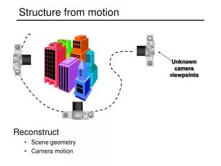
Structure from motion. Reconstruct Scene geometry Camera motion. Unknown camera viewpoints. Structure from motion. The SFM Problem Reconstruct scene geometry and camera motion from two or more images. Track 2D Features. Estimate 3D. Optimize (Bundle Adjust). Fit Surfaces.

Structure from motion
E N D
Presentation Transcript
Structure from motion • Reconstruct • Scene geometry • Camera motion Unknown camera viewpoints
Structure from motion • The SFM Problem • Reconstruct scene geometry and camera motion from two or more images Track 2D Features Estimate 3D Optimize (Bundle Adjust) Fit Surfaces SFM Pipeline
Structure from motion • Step 1: Track Features • Detect good features • corners, line segments • Find correspondences between frames • Lucas & Kanade-style motion estimation • window-based correlation
Structure Images Motion Structure from motion • Step 2: Estimate Motion and Structure • Simplified projection model, e.g., [Tomasi 92] • 2 or 3 views at a time [Hartley 00]
Structure from motion • Step 3: Refine Estimates • “Bundle adjustment” in photogrammetry
Structure from motion • Step 4: Recover Surfaces • Image-based triangulation [Morris 00, Baillard 99] • Silhouettes [Fitzgibbon 98] • Stereo [Pollefeys 99] Poor mesh Good mesh Morris and Kanade, 2000
Feature tracking • Problem • Find correspondence between n features in f images • Issues • What’s a feature? • What does it mean to “correspond”? • How can correspondence be reliably computed?
Feature detection • What’s a good feature?
Good features to track • Recall Lucas-Kanade equation: • When is this solvable? • ATA should be invertible • ATA should not be too small due to noise • eigenvalues l1 and l2 of ATA should not be too small • ATA should be well-conditioned • l1/ l2 should not be too large (l1 = larger eigenvalue) • These conditions are satisfied when min(l1, l2) > c
Feature correspondence • Correspondence Problem • Given feature patch F in frame H, find best match in frame I Find displacement (u,v) that minimizes SSD error over feature region • Solution • Small displacement: Lukas-Kanade • Large displacement: discrete search over (u,v) • Choose match that minimizes SSD (or normalized correlation)
Find displacement (u,v) that minimizes SSD error over feature region • Minimize with respect to Wx and Wy • Affine model is common choice [Shi & Tomasi 94] Feature distortion • Feature may change shape over time • Need a distortion model to really make this work
Tracking over many frames • So far we’ve only considered two frames • Basic extension to f frames • Select features in first frame • Given feature in frame i, compute position/deformation in i+1 • Select more features if needed • i = i + 1 • If i < f, go to step 2 • Issues • Discrete search vs. Lucas Kanade? • depends on expected magnitude of motion • discrete search is more flexible • How often to update feature template? • update often enough to compensate for distortion • updating too often causes drift • How big should search window be? • too small: lost features. Too large: slow
Incorporating dynamics • Idea • Can get better performance if we know something about the way points move • Most approaches assume constant velocity or constant acceleration • Use above to predict position in next frame, initialize search
Modeling uncertainty • Kalman Filtering (http://www.cs.unc.edu/~welch/kalman/ ) • Updates feature state and Gaussian uncertainty model • Get better prediction, confidence estimate • CONDENSATION (http://www.dai.ed.ac.uk/CVonline/LOCAL_COPIES/ISARD1/condensation.html ) • Also known as “particle filtering” • Updates probability distribution over all possible states • Can cope with multiple hypotheses
Approach • Predict position at time t: • Measure (perform correlation search or Lukas-Kanade) and compute likelihood • Combine to obtain (unnormalized) state probability Probabilistic Tracking • Treat tracking problem as a Markov process • Estimate p(xt | zt, xt-1) • prob of being in state xt given measurement zt and previous state xt-1 • Combine Markov assumption with Bayes Rule measurement likelihood (likelihood of seeing this measurement) prediction (based on previous frame and motion model)
prediction measurement posterior prediction Kalman filtering: assume p(x) is a Gaussian • Key • s = x (position) • o = z (sensor) initial state [Schiele et al. 94], [Weiß et al. 94], [Borenstein 96], [Gutmann et al. 96, 98], [Arras 98] Robot figures courtesy of Dieter Fox
Modeling probabilities with samples • Allocate samples according to probability • Higher probability—more samples
Measurement posterior CONDENSATION [Isard & Blake] Initialization: unknown position (uniform)
CONDENSATION [Isard & Blake] • Prediction: • draw new samples from the PDF • use the motion model to move the samples
Measurement posterior CONDENSATION [Isard & Blake]
Monte Carlo robot localization • Particle Filters [Fox, Dellaert, Thrun and collaborators]
CONDENSATION Contour Tracking • Training a tracker
CONDENSATION Contour Tracking • Red: smooth drawing • Green: scribble • Blue: pause
Structure from motion • The SFM Problem • Reconstruct scene geometry and camera positions from two or more images • Assume • Pixel correspondence • via tracking • Projection model • classic methods are orthographic • newer methods use perspective • practically any model is possible with bundle adjustment
image point projection matrix scene point image offset SFM under orthographic projection • Trick • Choose scene origin to be centroid of 3D points • Choose image origins to be centroid of 2D points • Allows us to drop the camera translation: More generally: weak perspective, para-perspective, affine
projection of n features in f images W measurement M motion S shape Key Observation: rank(W) <= 3 Shape by factorization [Tomasi & Kanade, 92] projection of n features in one image:
solve for known • Factorization Technique • W is at most rank 3 (assuming no noise) • We can use singular value decomposition to factor W: Shape by factorization [Tomasi & Kanade, 92]
Singular value decomposition (SVD) • SVD decomposes any mxn matrix A as • Properties • Σ is a diagonal matrix containing the eigenvalues of ATA • known as “singular values” of A • diagonal entries are sorted from largest to smallest • columns of U are eigenvectors of AAT • columns of V are eigenvectors of ATA • If A is singular (e.g., has rank 3) • only first 3 singular values are nonzero • we can throw away all but first 3 columns of U and V • Choose M’ = U’, S’ = Σ’V’T
solve for known • Factorization Technique • W is at most rank 3 (assuming no noise) • We can use singular value decomposition to factor W: • S’ differs from S by a linear transformation A: • Solve for A by enforcing metric constraints on M Shape by factorization [Tomasi & Kanade, 92]
Trick (not in original Tomasi/Kanade paper, but in followup work) • Constraints are linear in AAT: • Solve for G first by writing equations for every Pi in M • Then G = AAT by SVD (since U = V) Metric constraints • Orthographic Camera • Rows of P are orthonormal: • Weak Perspective Camera • Rows of P are orthogonal: • Enforcing “Metric” Constraints • Compute A such that rows of M have these properties
Factorization with noisy data • Once again: use SVD of W • Set all but the first three singular values to 0 • Yields new matrix W’ • W’ is optimal rank 3 approximation of W • Approach • Estimate W’, then use noise-free factorization of W’ as before • Result minimizes the SSD between positions of image features and projection of the reconstruction
Many extensions • Independently Moving Objects • Perspective Projection • Outlier Rejection • Subspace Constraints • SFM Without Correspondence
Extending factorization to perspective • Several Recent Approaches • [Christy 96]; [Triggs 96]; [Han 00]; [Mahamud 01] • Initialize with ortho/weak perspective model then iterate • Christy & Horaud • Derive expression for weak perspective as a perspective projection plus a correction term: • Basic procedure: • Run Tomasi-Kanade with weak perspective • Solve for i (different for each row of M) • Add correction term to W, solve again (until convergence)
Bundle adjustment • 3D → 2D mapping • a function of intrinsics K, extrinsics R & t • measurement affected by noise • Log likelihood of K,R,t given {(ui,vi)} • Minimized via nonlinear least squares regression • called “Bundle Adjustment” • e.g., Levenberg-Marquardt • described in Press et al., Numerical Recipes
Match Move • Film industry is a heavy consumer • composite live footage with 3D graphics • known as “match move” • Commercial products • 2D3 • http://www.2d3.com/ • RealVis • http://www.realviz.com/ • Show video
Closing the loop • Problem • requires good tracked features as input • Can we use SFM to help track points? • basic idea: recall form of Lucas-Kanade equation: • with n points in f frames, we can stack into a big matrix • Matrix on RHS has rank <= 3 !! • use SVD to compute a rank 3 approximation • has effect of filtering optical flow values to be consistent • [Irani 99]
References • C. Baillard & A. Zisserman, “Automatic Reconstruction of Planar Models from Multiple Views”, Proc. Computer Vision and Pattern Recognition Conf. (CVPR 99) 1999, pp. 559-565. • S. Christy & R. Horaud, “Euclidean shape and motion from multiple perspective views by affine iterations”, IEEE Transactions on Pattern Analysis and Machine Intelligence, 18(10):1098-1104, November 1996 (ftp://ftp.inrialpes.fr/pub/movi/publications/rec-affiter-long.ps.gz ) • A.W. Fitzgibbon, G. Cross, & A. Zisserman, “Automatic 3D Model Construction for Turn-Table Sequences”, SMILE Workshop, 1998. • M. Han & T. Kanade, “Creating 3D Models with Uncalibrated Cameras”, Proc. IEEE Computer Society Workshop on the Application of Computer Vision (WACV2000), 2000. • R. Hartley & A. Zisserman, “Multiple View Geometry”, Cambridge Univ. Press, 2000. • R. Hartley, “Euclidean Reconstruction from Uncalibrated Views”, In Applications of Invariance in Computer Vision, Springer-Verlag, 1994, pp. 237-256. • M. Isard and A. Blake, “CONDENSATION -- conditional density propagation for visual tracking”, International Journal Computer Vision, 29, 1, 5--28, 1998. (ftp://ftp.robots.ox.ac.uk/pub/ox.papers/VisualDynamics/ijcv98.ps.gz ) • S. Mahamud, M. Hebert, Y. Omori and J. Ponce, “Provably-Convergent Iterative Methods for Projective Structure from Motion”,Proc. Conf. on Computer Vision and Pattern Recognition, (CVPR 01), 2001. (http://www.cs.cmu.edu/~mahamud/cvpr-2001b.pdf ) • D. Morris & T. Kanade, “Image-Consistent Surface Triangulation”, Proc. Computer Vision and Pattern Recognition Conf. (CVPR 00), pp. 332-338. • M. Pollefeys, R. Koch & L. Van Gool, “Self-Calibration and Metric Reconstruction in spite of Varying and Unknown Internal Camera Parameters”, Int. J. of Computer Vision, 32(1), 1999, pp. 7-25. • J. Shi and C. Tomasi, “Good Features to Track”, IEEE Conf. on Computer Vision and Pattern Recognition (CVPR 94), 1994, pp. 593-600 (http://www.cs.washington.edu/education/courses/cse590ss/01wi/notes/good-features.pdf ) • C. Tomasi & T. Kanade, ”Shape and Motion from Image Streams Under Orthography: A Factorization Method", Int. Journal of Computer Vision, 9(2), 1992, pp. 137-154. • B. Triggs, “Factorization methods for projective structure and motion”, Proc. Computer Vision and Pattern Recognition Conf. (CVPR 96), 1996, pages 845--51. • M. Irani, “Multi-Frame Optical Flow Estimation Using Subspace Constraints”, IEEE International Conference on Computer Vision (ICCV), 1999 (http://www.wisdom.weizmann.ac.il/~irani/abstracts/flow_iccv99.html )