Probability: Basic Concepts and Applications in Archaeology
Explore frequentist and Bayesian approaches to probability, learn basic concepts like mutually exclusive events and conditional probabilities, and apply binomial theorem. Discover practical applications in archaeology.

Probability: Basic Concepts and Applications in Archaeology
E N D
Presentation Transcript
Questions • what is a good general size for artifact samples? • what proportion of populations of interest should we be attempting to sample? • how do we evaluate the absence of an artifact type in our collections?
“frequentist” approach • probability should be assessed in purely objective terms • no room for subjectivity on the part of individual researchers • knowledge about probabilities comes from the relative frequency of a large number of trials • this is a good model for coin tossing • not so useful for archaeology, where many of the events that interest us are unique…
Bayesian approach • Bayes Theorem • Thomas Bayes • 18th century English clergyman • concerned with integrating “prior knowledge” into calculations of probability • problematic for frequentists • prior knowledge = bias, subjectivity…
basic concepts • probability of event = p 0 <= p <= 1 0 = certain non-occurrence 1 = certain occurrence • .5 = even odds • .1 = 1 chance out of 10
basic concepts (cont.) • if A and B are mutually exclusive events: P(A or B) = P(A) + P(B) ex., die roll: P(1 or 6) = 1/6 + 1/6 = .33 • possibility set: sum of all possible outcomes ~A = anything other than A P(A or ~A) = P(A) + P(~A) = 1
basic concepts (cont.) • discrete vs. continuous probabilities • discrete • finite number of outcomes • continuous • outcomes vary along continuous scale
discrete probabilities .5 p .25 HH HT TT 0
.2 .2 p p .1 .1 0 0 continuous probabilities total area under curve = 1 but the probability of any single value = 0 interested in the probability assoc. w/ intervals
independent events • one event has no influence on the outcome of another event • if events A & B are independent then P(A&B) = P(A)*P(B) • if P(A&B) = P(A)*P(B) then events A & B are independent • coin flipping if P(H) = P(T) = .5 then P(HTHTH) = P(HHHHH) = .5*.5*.5*.5*.5 = .55 = .03
if you are flipping a coin and it has already come up heads 6 times in a row, what are the odds of an 7th head? .5 • note that P(10H) < > P(4H,6T) • lots of ways to achieve the 2nd result (therefore much more probable)
mutuallyexclusive events are not independent • rather, the most dependent kinds of events • if not heads, then tails • joint probability of 2 mutually exclusive events is 0 • P(A&B)=0
conditional probability • concern the odds of one event occurring, given that another event has occurred • P(A|B)=Prob of A, given B
e.g. • consider a temporally ambiguous, but generally late, pottery type • the probability that an actual example is “late” increases if found with other types of pottery that are unambiguously late… • P = probability that the specimen is late: isolated: P(Ta) = .7 w/ late pottery (Tb): P(Ta|Tb) = .9 w/ early pottery (Tc): P(Ta|Tc) = .3
conditional probability (cont.) • P(B|A) = P(A&B)/P(A) • if A and B are independent, then P(B|A) = P(A)*P(B)/P(A) P(B|A) = P(B)
Bayes Theorem • can be derived from the basic equation for conditional probabilities
application • archaeological data about ceramic design • bowls and jars, decorated and undecorated • previous excavations show: • 75% of assemblage are bowls, 25% jars • of the bowls, about 50% are decorated • of the jars, only about 20% are decorated • we have a decorated sherd fragment, but it’s too small to determine its form… • what is the probability that it comes from a bowl?
can solve for P(B|A) • events:?? • events: B = “bowlness”; A = “decoratedness” • P(B)=??; P(A|B)=?? • P(B)=.75; P(A|B)=.50 • P(~B)=.25; P(A|~B)=.20 • P(B|A)=.75*.50 / ((.75*50)+(.25*.20)) • P(B|A)=.88
Binomial theorem • P(n,k,p) • probability of k successes in n trialswhere the probability of success on any one trial is p • “success” = some specific event or outcome • k specified outcomes • n trials • p probability of the specified outcome in 1 trial
where n! = n*(n-1)*(n-2)…*1(where n is an integer) 0!=1
binomial distribution • binomial theorem describes a theoretical distribution that can be plotted in two different ways: • probability density function (PDF) • cumulative density function (CDF)
probability density function (PDF) • summarizes how odds/probabilities are distributed among the events that can arise from a series of trials
ex: coin toss • we toss a coin three times, defining the outcome head as a “success”… • what are the possible outcomes? • how do we calculate their probabilities?
coin toss (cont.) • how do we assign values to P(n,k,p)? • 3 trials; n = 3 • even odds of success; p=.5 • P(3,k,.5) • there are 4 possible values for ‘k’, and we want to calculate P for each of them “probability of k successes in n trialswhere the probability of success on any one trial is p”
practical applications • how do we interpret the absence of key types in artifact samples?? • does sample size matter?? • does anything else matter??
example • we are interested in ceramic production in southern Utah • we have surface collections from a number of sites • are any of them ceramic workshops?? • evidence: ceramic “wasters” • ethnoarchaeological data suggests that wasters tend to make up about 5% of samples at ceramic workshops
one of our sites 15 sherds, none identified as wasters… • so, our evidence seems to suggest that this site is not a workshop • how strong is our conclusion??
reverse the logic: assume that it is a ceramic workshop • new question: • how likely is it to have missed collecting wasters in a sample of 15 sherds from a real ceramic workshop?? • P(n,k,p) [n trials, k successes, p prob. of success on 1 trial] • P(15,0,.05) [we may want to look at other values of k…]
how large a sample do you need before you can place some reasonable confidence in the idea that no wasters = no workshop? • how could we find out?? • we could plot P(n,0,.05) against different values of n…
50 – less than 1 chance in 10 of collecting no wasters… • 100 – about 1 chance in 100…
so, how big should samples be? • depends on your research goals & interests • need big samples to study rare items… • “rules of thumb” are usually misguided (ex. “200 pollen grains is a valid sample”) • in general, sheer sample size is more important that the actual proportion • large samples that constitute a very small proportion of a population may be highly useful for inferential purposes
the plots we have been using are probability density functions (PDF) • cumulative density functions (CDF) have a special purpose • example based on mortuary data…
Pre-Dynastic cemeteries in Upper Egypt Site 1 • 800 graves • 160 exhibit body position and grave goods that mark members of a distinct ethnicity (group A) • relative frequency of 0.2 Site 2 • badly damaged; only 50 graves excavated • 6 exhibit “group A” characteristics • relative frequency of 0.12
expressed as a proportion, Site 1 has around twice as many burials of individuals from “group A” as Site 2 • how seriously should we take this observation as evidence about social differences between underlying populations?
assume for the moment that there is no difference between these societies—they represent samples from the same underlying population • how likely would it be to collect our Site 2 sample from this underlying population? • we could use data merged from both sites as a basis for characterizing this population • but since the sample from Site 1 is so large, lets just use it …
Site 1 suggests that about 20% of our society belong to this distinct social class… • if so, we might have expected that 10 of the 50 sites excavated from site 2 would belong to this class • but we found only 6…
how likely is it that this difference (10 vs. 6) could arise just from random chance?? • to answer this question, we have to be interested in more than just the probability associated with the single observed outcome “6” • we are also interested in the total probability associated with outcomes that are more extreme than “6”…
imagine a simulation of the discovery/excavation process of graves at Site 2: • repeated drawing of 50 balls from a jar: • ca. 800 balls • 80% black, 20% white • on average, samples will contain 10 white balls, but individual samples will vary
by keeping score on how many times we draw a sample that is as, or more divergent (relative to the mean sample) than what we observed in our real-world sample… • this means we have to tally all samples that produce 6, 5, 4…0, white balls… • a tally of just those samples with 6 white balls eliminates crucial evidence…
we can use the binomial theorem instead of the drawing experiment, but the same logic applies • a cumulative density function (CDF) displays probabilities associated with a range of outcomes (such as 6 to 0 graves with evidence for elite status)
so, the odds are about 1 in 10 that the differences we see could be attributed to random effects—rather than social differences • you have to decide what this observation really means, and other kinds of evidence will probably play a role in your decision…

