Download

1 / 33
330 likes | 457 Vues
COP 3502: Computer Science I Spring 2004 – Note Set 12 – Searching and Sorting – Part 3. Instructor : Mark Llewellyn markl@cs.ucf.edu CC1 211, 823-2790 http://www.cs.ucf.edu/courses/cop3502/spr04. School of Electrical Engineering and Computer Science

E N D
COP 3502: Computer Science I Spring 2004 – Note Set 12 – Searching and Sorting – Part 3 Instructor : Mark Llewellyn markl@cs.ucf.edu CC1 211, 823-2790 http://www.cs.ucf.edu/courses/cop3502/spr04 School of Electrical Engineering and Computer Science University of Central Florida
Quicksort is another recursive sorting algorithm. It picks an element from the list and uses it to divide the list into two parts. It then places every element which is smaller than the selected element into the first part and every element which is larger than the selected element is placed into the second part. Before we look at Quicksort in any detail, we’ll first examine a related problem that will help you understand how and why Quicksort works. QuickSort
We’ve already examined the problem of searching a list for a specific target element. There is a closely related problem to this called selection. The selection problem is similar to the searching problem except where searching is concerned with finding a specific target element in the list, selection is concerned with finding an element which exhibits a certain property, such as the largest, smallest, or median value. In general, the selection problem solves the problem of finding the kthlargest value in a list. Problem Related to QuickSort: Selection
One way to solve the selection problem would be to sort the list in decreasing order, and then the kth largest value would be in position k. However, this is a lot more work that we really need to do, because we don’t really care about the values that are smaller than the one we want. A related technique would be to find the largest value and then move it to the last location in the list. If we again look for the largest value in the list ignoring the value we already found, we get the second largest value, which can be moved to the next to the last location in the list. This process would repeat until we had found the kth largest value which would occur on the kth pass. The algorithm for this is shown on the next page. Problem Related to QuickSort: Selection (cont.)
FindKthLargest Algorithm FindKthLargest (list, n, k) // list the list of elements to look through // n the number of elements in the list // k the element to select for (i = 1; i <= k, i++) { largest = list[1]; largestLocation = 1; for ( j = 2, j <= n-(i-1); j++){ if listpj[ > largest then { largest = list[j]; largestLocation = j; } } swap( list[n-(i-1)], list[largestLocation]); } end.
On the first pass a total of n-1 comparisons would be made. The second pass would total n-2 comparisons, and so on. On the kth pass a total of n-k comparisons would occur. This gives: Note that this equation also tells us that if k is greater than n/2, it would be faster for look for the n-kth smallest value. This algorithm is reasonably efficient for values of k that are close to either end of the list, but there is a more efficient way to accomplish this process for values of k that are close to the middle of the list. Can you think of a technique that would accomplish this? Complexity of FindKthLargest
Since we are only interested in the kth largest value, we don’t really need to know the exact position for the values that are the largest through the k-1st largest; we only need to know that they are larger...their position in the list is irrelevant. If we choose an element from the list and partition the list into two distinct parts, one containing those elements that are larger than the chosen element and the other containing those elements that are smaller than the chosen element. The chosen element will wind up in some position p in the list. This will mean that the chosen element is the pth largest element in the list. Complexity of FindKthLargest (cont.)
To accomplish this partitioning, we’ll need to compare the chosen element with all of the other elements, requiring n-1 comparisons. If we are lucky and p = k, then we’re done. If k < p, then we need a smaller value to partition on (a smaller p) and we’ll repeat the process on a second partitioning. If k > p, then we need a larger value to partition on (a larger p) and we’ll use the first partition, but we’ll need to reduce the value of k by the number of values we’ve eliminated in the larger partition. The following few pages illustrates this technique. Complexity of FindKthLargest (cont.)
9 13 46 55 6 23 44 88 95 Complexity of FindKthLargest (cont.) Nomenclature for list elements 1st largest nth largest 2nd largest (n-1)th largest 3rd largest (n-2)th largest pth largest. In this case p=k = 5 This element is positioned k elements from the high end of the list.
23 9 55 13 95 46 88 55 Complexity of FindKthLargest (cont.) Suppose we are looking for the 7th largest element (k= 7) Initial List 6 23 44 88 95 chosen element First partitioning 6 9 13 44 46 chosen element We made a good “guess” and the chosen element winds up as the 7th largest element which is what we wanted. Element 55 winds up in 7th position, so k = p =7.
44 46 9 55 13 55 95 46 95 88 88 55 First partitioning 6 9 13 23 46 We made a poor “guess” and the chosen element winds up as the 3rd largest element (p = 3), which is smaller than we wanted. Since k > p, we’ll do a second partitioning of the larger numbers. Complexity of FindKthLargest (cont.) Suppose we are looking for the 6th largest element (k= 6) Initial List 6 23 44 88 95 chosen element chosen element Second partitioning 6 9 13 23 44 We made a good “guess” this time and the chosen element winds up as the 6th largest element. Since p=k=6, we are done. chosen element ignore these elements this time
Suppose we are looking for the 2nd largest element Initial List 6 23 44 88 95 46 9 46 88 88 13 46 95 95 55 55 55 chosen element First partitioning 6 9 23 44 13 chosen element We made a poor “guess” and the chosen element winds up as the 6th largest element (p=6) which is larger than what we wanted. Since k < p, we’ll repartition, but select an element smaller than 46. Complexity of FindKthLargest (cont.) Second partitioning 6 9 13 44 23 new chosen element We made a good “guess” the second time and the chosen element winds up as the 2nd largest element (p=2) which is what we wanted. ignore these elements this time
Recursive FindKthLargest Algorithm KthLargestRecursive (list, n, k) // list the list of elements to look through // start the index of the first element to consider // end the index of the last element to consider // k the element of the list we want if start < end { Partition( list, start, end, middle); if middle = k return list[middle]; else if k < middle return KthLargestRecursive( list, middle+1, end, k); else return(KthLargestRecursive( list, start, middle-1, k-middle); } end.
If we assume that on average the partitioning process will divide the list into two roughly equal halves, then approximately: n + n/2 + n/4 + n/8 + … + 1 will be be necessary. This is about 2n comparisons. So the process is linear and independent of k. Complexity of KthLargestRecursive
Quicksort is another recursive sorting algorithm. It picks an element from the list, called the pivot element, and uses it to divide the list into two parts. The first part contains all of the elements that are smaller than the pivot element and the second part of the list contains all of the elements that are larger than the pivot element. This process is similar to the one we just saw utilized when searching for the kth largest element in a list. The only difference is that quicksort applies the technique recursively to both parts of the list. Quicksort is a very efficient sort on average, although its worst case performance is identical to insertion sort and bubble sort at O(n2). Quicksort
Once the pivot element is selected (more on this later) the list is rearranged so that elements smaller than the pivot element are moved before it and elements larger than it are moved after the pivot element. The elements in each of the two parts of the list are not put in order. If the pivot element winds up in location i, all we know for certain is that elements in locations 1 through i-1 are smaller than the pivot element and those in locations i+1 through n are larger than the pivot element. Once this is done, quicksort is called recursively on these two parts. Quicksort (cont.)
If quicksort is called with a list containing one element, it does nothing (base case) because a one-element list is sorted by default. Because the determination of the pivot element and the movement of the elements into the proper section do all the work, the main quicksort algorithm just needs to keep track of the bounds of these two sections of the list. Further, because splitting the list into two parts is where the keys are moved around, all the sorting work is done on the way down in the recursive process. IMPORTANT NOTE: This is exactly opposite of merge sort, which does its work on the way back up in the recursive process. The algorithm for quicksort is shown on the next page. Quicksort (cont.)
Quicksort Algorithm Quicksort (list, first, last) // list the list of elements to be sorted // first the index of the first element in the part of the list to sort // last the index of the last element to in the part of the list to sort. if first < last { pivot = PivotList( list, first, last); Quicksort( list, first, pivot-1); Quicksort( list, pivot+1, last); } end.
PivotList Algorithm PivotList (list, first, last) // list the list of elements to work with // first the index of the first element // last the index of the last element pivotvalue = list[first]; pivotpoint = first; for (index = first+1, index <= last, index++) { if list[index] < pivotvalue { pivotpoint = pivotpoint+1; swap( list[pivotpoint+1, list[index]); } } //move pivot value into correct place in list swap( list[first], list[pivotpoint]); return pivotpoint; end.
Relationship between indices and element in Algorithm PivotList pivot < pivot >= pivot unknown pivot point index first last
There are at least two versions of the PivotList function. The version shown on page 19 is easy to program and understand . There is another version which is more complicated to write but is faster than the version on page 19. I’ll show you this version at the end of this section of notes, but we’ll do our analysis of the quicksort algorithm using the simple partitioning algorithm from page 19. The diagram on page 20 illustrates how the PivotList algorithm partitions the list into two distinct sublists. Note that this simple algorithm simply chooses the first element in the list as the pivot element. Splitting the List for Quicksort
Since the first element in the list is selected as the pivot element, the location of the pivot element is initially set to 1. The algorithm then moves through the list comparing this pivot element to the rest of the elements. Whenever it finds an element that is smaller than the pivot element, it will increment the pivot point and then swap this element into the pivot point location. After some of the elements have been compared to the pivot inside the loop, there will be four basic parts to the list as shown by the diagram on page 20. Splitting the List for Quicksort (cont.)
The first part of the list is simply the pivot element in the first location. The second part of the list is from location first+1 through the pivot location and will consist of all the elements that have been compared which are smaller than the pivot element. The third part of the list is from the location after the pivot location through the loop index and will consist of all compared elements which are larger than the pivot element. The fourth part of the list consists of all the elements which have not yet been compared. These four parts are illustrated in the diagram on page 20. Splitting the List for Quicksort (cont.)
When PivotList is called with a list of n elements, it does n-1 comparisons as it compares the pivot value with every other element in the list. Since we know that quicksort is a divide and conquer algorithm, we would be correct in assuming that the best case performance would occur when PivotList creates two equal sized parts to the original list. The worst case performance would then logically occur when the two parts of the list are of drastically different sizes. The worst case occurs when one part has no elements and the other part contains n-1 elements. If the same thing were to occur each time we partitioned the list we would remove only one element from the list on each recursive call (the pivot element). Worst Case Analysis for Quicksort
Given this worst case scenario, PivotList would do a number of comparisons given by: What original ordering of the elements would cause this sort of behavior? If each pass chooses the first element, that element must be the smallest (or largest). A list that is already sorted is one arrangement that would cause this worst case performance. All of the other sorts that we have seen, the worst case and average cases have been about the same (equal asymptotically), but as we are about to see, this is not the case for quicksort. Worst Case Analysis for Quicksort(cont.)
All of the work of quicksort is done by PivotList, so here is where we need to look for the average case. It is possible for each of the n locations in the list to be the location of the pivot element. So we need to see what happens for each of these possibilities and average the results. When looking at the worst case, we saw that for a list of n elements, n-1 comparisons were necessary to divide the list. There is no work to put the lists back together. Also notice that when PivotList returns a value of p, quicksort is called recursively with lists of p-1 and n-p elements. Our average case needs to look at all n possible values for p, which gives: Average Case Analysis for Quicksort
If you look closely at the summation, you will notice the first term is used with values from 0 through n-1 and the second term is used with values from n-1 down to 0. This means that the summation adds up every value of the average from 0 to n-1 twice. This leads to the following simplification: Average Case Analysis for Quicksort (cont.)
This is a very complicated form of a recurrence relation because it depends on not just one smaller value of the average, but rather on every smaller value for the average! There are two basic ways to solve such a recurrence relation: (1) come up with an educated guess for the answer and then prove that this answer does satisfy the recurrence relation, or (2) look at the equations for both average(n) and average(n-1). Since these two equations differ by only a few terms: Computing average(n) n and average(n-1)(n-1) gets rid of the fractions which gives: Average Case Analysis for Quicksort (cont.)
Average Case Analysis for Quicksort (cont.) Subtracting the second equation from the first and simplifying gives: Adding average(n-1) (n-1) to both sides, we get:
Average Case Analysis for Quicksort (cont.) This gives our final recurrence relation: Solving this is not too difficult but does require care because all of the terms on the right-hand side of the equation. If you work through all of the details (we’re not going to!), you’ll see the final result is:
Quicksort is the fastest known comparison based sorting algorithm. Summary of Quicksort
A faster alternative for the PivotList function would be to have two indices into the list. The first moves up from the low end of the list and the second moves down from the high end of the list. The main loop of the algorithm will advance the lower index until a greater value than the pivot element is found, and the upper index is moved until a value less than the pivot element is found. When this situation occurs these two elements are swapped. The process repeats until the two indices cross over each other. These inner loops are very fast because the overhead of checking for the end of the list is eliminated, but one problem is that an extra swap occurs when the indices cross. Alternative PivotList Function
PivotList Algorithm FastPivotList (list, first, last) // list the list of elements to work with // first the index of the first element // last the index of the last element pivotvalue = list[first]; lower = first; upper = last +1; do do upper = upper–1 until list[upper] <= pivotvalue do lower = lower+1 until list[lower] >= pivotvalue swap( list[upper], list[lower]) until lower >= upper //undo the extra exchange swap( list[upper], list[lower]); //move pivot point into correct location swap( list[first], list[upper]) return upper end. This algorithm requires that the list have one extra location to hold a special sentinel value which is larger than all of the valid key fields in the list.