Download
1 / 29
290 likes | 469 Vues
The Invisible Hand and the Banking Trade: seigniorage , risk-shifting, and more. By Marcus Miller and Lei Zhang University of Warwick . ‘There are few ways a man may be more innocently employed than in getting money’. Samuel Johnson (1775, letter to his printer). Peyton Young.

E N D
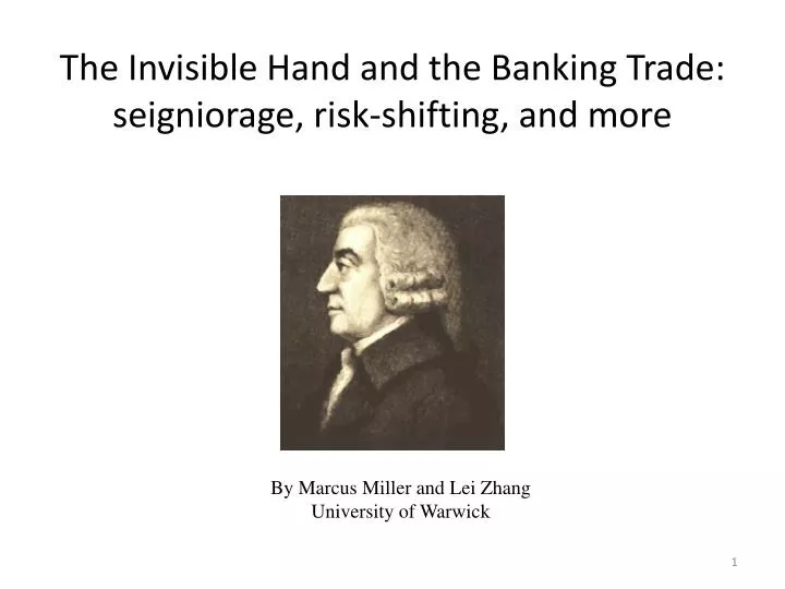
The Invisible Hand and the Banking Trade: seigniorage, risk-shifting, and more By Marcus Miller and Lei Zhang University of Warwick
‘There are few ways a man may be more innocently employed than in getting money’. Samuel Johnson (1775, letter to his printer) Peyton Young Joseph Stiglitz Two economists who examined the operation of the invisible hand in the banking trade.
Summary • Start with classic Diamond –Dybvig model of banking (as in Allen and Gale, 2007) • Add monopoly power – private seigniorage • Analyse market structure – “take it or leave it” vs. Cournot Nash monopoly and oligopoly. • Add a productivitymiracle restricted to the private sector, as for star traders for example. • Add gambling with ‘tail risk’ where the upside is perceived but downside is not (as in Foster and Young, 2010 which goes further than Hellman Murdock and Stiglitz, 2000). • Implications for Gini coefficient • DD + HMS – RE = this paper
Summary - continued • Explicit results for extreme risk aversion- competitive equil, monopoly, franchise value, No Gambling Condition, etc. • How franchise value can check gambling thru ‘skin in the game’(TBTG); but bailout prospect can offset this (TBTF), leading to U-shaped prudential frontier. • How Vickers Report aims to check excess risk- taking and bailouts
Late Consumption The Classic Diamond-Dybvig Model of Banking: the perfectly competitive outcome as in DD (1983) Banks’ No-Profit Constraint Inter-temporal optimality R N C Consumers’ Offer Curve Constant Expected Utility 1 Early Consumption
Late Consumption Adding seigniorage: monopoly outcomes Banks’ No-Profit Constraint Inter-temporal optimality S R N C M Consumers’ Offer Curve Monopoly profits = private seigniorage Constant Expected Utility T Two measures: “Take it or leave it”: as at T Standard monopoly: as at M 1 Early Consumption
2. Coalition-proof concentration in banking Inter-temporal efficiency condition N B M D C X Participation constraint
Monopoly profits increase with increasing risk aversion (ref. Miller, Zhang and Li,2013)
The demand for money and the flow of private seigniorage M C Marginal cost Demand Marginal revenue
Bank profits: productivity miracle or mirage? Late Consumption New No-Profit Constraint A productivity improvement in banking: competition vs. monopoly S’ Inter-temporal efficiency condition N C’ R M’ M C Offer Curve Participation Constraint Early Consumption 1
A “productivity miracle” - or risk-shifting? Between 1970 and 2008, the share of banking in economy-wide profits rose 10 fold (from 1.5% to 15%). Haldane et al. (2010) Source: Haldane et al. (2010, p.68) Gross operating surplus of UK private financial corporations (% of total)
Source: Robert Reich, Berkley, CA. (now starring in Inequality for all)
1 P Gambling and Gini Coefficient σ:the fraction of the population owning shares in the all-deposit bank. ω: the consumption bundle available to depositors under monopoly banking. ω(1+μ): the consumption available to the depositors who are also shareholders enjoying the monopoly premium, μ, in this case Gini coefficient: Cumulative fraction of income When the bank gambles, the premium paid to owner-managers will of course rise, say to , shifting the Lorenz curve to in the figure. i.e. the area OLP divided by O1P in the diagram. O 1-σ 1 Cumulative fraction of population from lowest to highest incomes Rising incomes in financial services and income inequality
Commercial banking with extreme risk aversion (Leontief preferences). The competitive contract, , is shown at the point labelled C in the Figure where =0.5.
Perfect Competition* Leontief preferences imply: (6) with prudent investment the zero profit condition is: (7) Together these yield the competitive contract, , see figure. With gambling, the zero profit condition becomes: (8) So solving for the deposit contract using (6) and (8) yields (9) To avoid gambling under perfect competition, one has to choose k such that . This implies the critical capital requirement of (10) * Equation numbers refer to ‘The invisible Hand and the banking trade’, Miller and Zhang (2013)
Monopoly With extreme risk aversion, where long returns are R, profits without gambling will be at a maximum at the point shown as M, where the flow of seigniorage is: (11) When this is capitalised at a discount rate of δ, this provides the franchise value of the monopoly bank, (12) Assume there is a gamble available with high and low payoffs, RH>R>RL,and probabilities respectively, and that it is a mean–preserving spread relative to the return of R , so = R . With the monopoly contract of (1,1) as before, the expected monopoly profit (measured at date 2) will be: )] +(1-π)0, So (13)
Do Monopoly Profits Increase with Gambling? It may seem obvious that keeping the upside of the gamble and passing the downside on to taxpayers will raise profits. But let us check this is the case, for < . > ? = > ? -(-? (() QED
The No Gambling Condition for a monopolist For the franchise value V to prevent gambling, it is necessary that: . (14) For checking gambling, capital requirements may be imposed. Adding the risk of losing regulatory capital at end of period, expected profits become: So NGC is . (15) (This can be rewritten as, indicating that Rkis a perfect substitute for .) The critical value of k can be found when (15) is an equality, yielding (16)
“Looting” and “gambling” Akerlof and Romer (1993) on looting: If owners can pay themselves dividends greater than the true economic value of the thrift, they will do so, even if this requires that they invest in projects with negative net present value. … [But] when they can take out more than the thrift is worth, they cause the thrift to default on its obligations in period 2. If they are going to default, the owners do not care if the investment project has a negative net present value because they government suffers all of the losses on the project. (pp.10) Compare this to HMS on incentives for banks to gamble where the NGC is “the one period rent that the bank expects to earn from gambling must be less than the franchise value that the bank gives up if the gamble fails” (pp. 152-153). If not, the owners/ managers of the bank go ahead to extract current value, even though this risks bankruptcy. Q: Is the HMS analysis a kind of looting?
Monopoly with Bailout prospect, β. How does the prospect of a bailout, where the owners/ managers of the bank lose their ‘skin in the game’ (k) but not the franchise value, affect the capital requirement? . (17) Note that a greater prospect of bailout calls for higher k. When β = 0, the above NGC reverts to that without bailout. When β = 1, so the monopolist is sure to be bailed out, the NGC becomes the critical level of capital requirements is: (18)
Tail-risk and nasty surprises Foster and Young (2010) explore one way of capturing unexpected developments, namely by the use of probability distributions associated with extreme events -- fat-tailed distributions with ‘tail risk’, consistent with the very rare occurrence of disastrously bad returns. They show that, by using derivatives in a setting of asymmetric information, such downside risk in investment portfolios can be concealed from outside observers for considerable periods of time: unknown to outsiders, investors can mis-sell puts offering insurance against rare but catastrophic events. ‘Tail risk’ refers to the events which lie in the tail of the distribution, at least three times the standard deviation away from the mean. For the normal distribution, commonly used in finance, 99.7% of the distribution lies within 3 standard deviations of the mean, so the likelihood of being in one of the tails is: (1- 99.7)/2 = 0.0015, i.e. 1.5 in 1000. For the “fat tailed” binomial distribution, ‘tail risk’ occurs when the difference between the mean return and that in the low state, , is at least three times the standard deviation, . As may readily be established, a sufficient condition for tail risk in the binomial is so the probability of the bad state is 0.1, i.e. 1 in 10.So people who believe the world is normally distributed are in for a nasty surprise!
No Gambling Outcomes with risk aversion with Leontief preferences Notes:
Gambling Outcomes with risk aversion with Leontief preferences Notes:; πδ=0.81.
Regulatory Capital, % Bailouts and moral hazard Prudent Banking Gambling L UK R TBTG TBTF Crisis Region k0 a b B Gambling M Concentration, 1/N TBTG, TBTF and the U-shaped region of prudent banking
Ring-fencing, electric fencing, and all that: the Report of the ICB
R Regulatory Capital Prudent Banking Reduced incentive to Bailout L L′ R′ Risk Prohibition & Monitoring Higher capital requirements and more competition Concentration Regulatory Reform in the UK: in brief
References • Allen, F. and Gale, D. (2007), Understanding Financial Crises, New York: Oxford University Press. • Diamond, D.W. and Dybvig, P.H. (1983), ‘Bank Runs, Deposit Insurance, and Liquidity’. Journal of Political Economy, 91(3), 401–419. • Haldane, A., Brennan, S. and Madouros, V. (2010), ‘What is the Contribution of the Financial Sector: Miracle or Mirage?’, The Future of Finance: the LSE report, Chapter 2. London: LSE. • Hellmann, T. F., Murdock, K. C. and Stiglitz, J. E. (2000), ‘Liberalization, Moral Hazard in Banking, and Prudential Regulation: Are Capital Requirements Enough?’, American Economic Review, 90(1), 147-165. • Foster D. P. and Young, P. (2010), ‘Gaming Performance Fees by Portfolio Managers’. The Quarterly Journal of Economics, 125(4), 1435-1458. • Miller, M., Zhang, L. and Li, H. 'When bigger isn't better: bailouts and bank reform‘, Oxford Economic Papers, forthcoming, April 2013.
Looting: The Economic Underworld of Bankruptcy for Profit George Akerlof and Paul Romer, 1993 Bankruptcy for profit will occur if poor accounting, lax regulation, or low penalties for abuse give owners an incentive to pay themselves more than their firms are worth and then default on their debt obligations. Bankruptcy for profit occurs most commonly when a government guarantees a firm's debt obligations. The normal economics of maximizing economic value is re- placed by the topsy-turvy economics of maximizing current extractable value, which tends to drive the firm's economic net worth deeply negative. Because of this disparity between what the owners can capture and the losses that they create, we refer to bankruptcy for profit as looting. (pp.2-3)