• URL: .../publications/courses/ece_8423/lectures/current/lecture_08.ppt
120 likes | 387 Vues
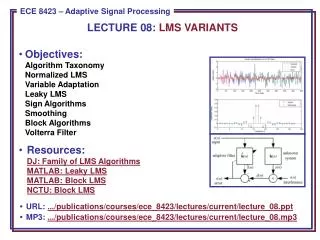
LECTURE 08: LMS VARIANTS. Objectives: Algorithm Taxonomy Normalized LMS Variable Adaptation Leaky LMS Sign Algorithms Smoothing Block Algorithms Volterra Filter Resources: DJ: Family of LMS Algorithms MATLAB: Leaky LMS MATLAB: Block LMS NCTU: Block LMS.

• URL: .../publications/courses/ece_8423/lectures/current/lecture_08.ppt
E N D
Presentation Transcript
LECTURE 08: LMS VARIANTS • Objectives:Algorithm TaxonomyNormalized LMSVariable AdaptationLeaky LMSSign AlgorithmsSmoothingBlock AlgorithmsVolterra Filter • Resources:DJ: Family of LMS AlgorithmsMATLAB: Leaky LMSMATLAB: Block LMSNCTU: Block LMS • URL: .../publications/courses/ece_8423/lectures/current/lecture_08.ppt • MP3: .../publications/courses/ece_8423/lectures/current/lecture_08.mp3
Algorithm Taxonomy • Thus far we have focused on: • Adaptive algorithm: LMS • Criterion: Least-squares • Iterative: Steepest descent • Implementation: Tapped delay line • and this doesn’t even includestatistical methods for feature andmodel adaptation. • There are many alternative optimizationcriteria (including ML methods). For example: Least Mean Fourth (LMF) Algorithm: N=2
Normalized LMS • The stability, convergence and steady-state properties of the LMS algorithm are directly influenced by the length of the filter and the power of the input signal. We can normalize the adaptation constant with respect to these: • We can estimate the power using a time average: • The update equations become: • We can add a small positive constant to avoid division by zero: • For the homogeneous problem ( ), it can be shown that: • For zero-mean Gaussian inputs, it can be shown to converge in the mean.
Variable Adaptation Rate • Another variation of the LMS algorithm is to use an adaptation constant that varies as a function of time: • This problem has been studied extensively in the context of neural networks. Adaptation can be implemented using a constant proportional to the “velocity” or “acceleration” of the error signal. • One extension of this approach is the Variable Step algorithm: • This is a generalization in that each filter coefficient has its own adaptation constant. Also, the adaptation constant is a function of time. • The step sizes are determined heuristically, such as examining the sign of the instantaneous gradient:
The Leaky LMS Algorithm • Consider an LMS update modified to include a constant “leakage” factor: • Under what conditions would it be advantageous to employ such a factor? • What are the drawbacks of this approach? • Substituting our expression for e(n) in terms of d(n) and rearranging terms: • Assuming independence of the filter and the data vectors: • It can be shown: • There is a bias from the LMS solution,R-1g, that demonstrates leakage is a compromise between bias and coefficient protection.
Sign Algorithms • To decrease the computational complexity, it is also possible to update the filter coefficients using just the sign of the error: • Pilot LMS, or Signed Error, or Sign Algorithm: • Clipped LMS or Signed Regressor: • Zero-Forcing LMS or Sign-Sign: • The algorithms are useful in applications where very high-speed data is being processed, such as communications equipment. • We can also derive these algorithms using a modified cost function: • The Sign-Sign algorithm is used in the CCITT ADPCM standard.
Smoothing of LMS Gradient Estimates • The gradient descent approach using an instantaneous sampling of the error signal is a noisy estimate. It is a tradeoff between computational simplicity and performance. • We can define an Averaged LMS algorithm: • A more general form of this uses a low-pass filter: • The filter can be FIR or IIR. • A popular variant of this approach is known as the Momentum LMS filter: • A nonlinear approach, known as the Median LMS (MLMS) Algorithm: • There are obviously many variants of these types of algorithms involving heuristics and higher-order approximations to the derivative.
The Block LMS (BLMS) Algorithm • There is no need to update coefficients every sample. We can update coefficients every N samples and use a block update for the coefficients: • The BLMS algorithm requires (NL+L) multiplications per block compared to (NL+N) per block of N points for the LMS. • It is easy to show that the convergence is slowed by a factor of N for the block algorithm, but on the other hand it uses excessive smoothing. • The block algorithm produces a different result than the per-sample updates (the two algorithms do not produce the same result), but the results are sufficiently close. • In many real applications, block algorithms are preferred because they fit better with hardware constraints and significantly reduce computations.
The LMS Volterra Filter • A second-order digital Volterra filter is defined as: • where f(1)(j) are the usual linear filter coefficients, and f(2)(j1,j2) are the L(L+1)/2 quadratic coefficients. • We can define the update equations in a manner completely analogous to the standard LMS filter: • Not surprisingly, one form of the solution is:
The LMS Volterra Filter (Cont.) • The correlation matrix, R, is defined as: • The extended cross-correlation vector is given by: • An adaptive second-order Volterra filter can be derived: • Once the basic extended equations have been established, the filter functions much like our standard LMS adaptive filter.
Summary • There are many types of adaptive algorithms. The LMS adaptive filter was have previously discussed is just one implementation. • The gradient descent algorithm can be approximated in many ways. • Coefficients can be updated per sample or on a block-by-block basis. • Coefficients can be smoothed using a block-based expectation. • Filters can exploit higher-order statistical information in the signal(e.g., the Volterra filter).