Download
1 / 40
400 likes | 513 Vues
This work delves into the stochastic geometry of turbulence, highlighting its complex characteristics through the lens of fractals and multi-fractals. By examining energy cascades and Kolmogorov scaling, we reveal how turbulence deviates from equilibrium, illustrating its irregular temporal and spatial patterns. The discussion encompasses various mathematical models, including the Euler equation and the Navier-Stokes equations, emphasizing the role of isolines in passive scalar fields in turbulent flows. Our findings suggest conformal invariance and the intricacies of vorticity isolines across different cascading regimes.

E N D
Stochastic geometry of turbulence Gregory Falkovich Weizmann Institute D. Bernard, G. Boffetta, Celani, S. Musacchio, K. Turitsyn,M. Vucelja APS meeting, 28 February 2012
Fractals, multi-fractals and God knows what depends neither on q nor on r - fractal depends on q – multi-fractal depends on r - God knows what
Turbulence is a state of a physical system with many degrees of freedom deviated far from equilibrium. It is irregular both in time and in space. Energy cascade and Kolmogorov scaling Transported scalar (Lagrangian invariant)
Full level set is fractal with D = 2 - ζ What about a single isoline? Random Gaussian Surfaces
Family of transport-type equations m=2 Navier-Stokes m=1 Surface quasi-geostrophic model, m=-2 Charney-Hasegawa-Mima model Electrostatic analogy: Coulomb law in d=4-m dimensions
This system describes geodesics on an infinitely-dimensional Riemannian manifold of the area-preserving diffeomorfisms. On a torus,
Add force and dissipation to provide for turbulence (*) lhs of (*) conserves
Kraichnan’s double cascade picture Q P k pumping
Boundary • Frontier • Cut points perimeter P Bernard, Boffetta, Celani &GF, Nature Physics 2006, PRL2007
Scalar exponents ζ of the scalar field (circles) and stream function (triangles), and universality class κ for different m ζ κ
M Vucelja , G Falkovich & K S Turitsyn Fractal iso-contours of passive scalar in two-dimensional smooth random flows. J Stat Phys 147 : 424–435 (2012)
Conclusion Within experimental accuracy, isolines of advected quantities are conformal invariant (SLE) in turbulent inverse cascades. Why? Vorticity isolines in the direct cascade are multi-fractal. Isolines of passive scalar in the Batchelor regime continue to change on a time scale vastly exceeding the saturation time of the bulk scalar field. Why?