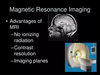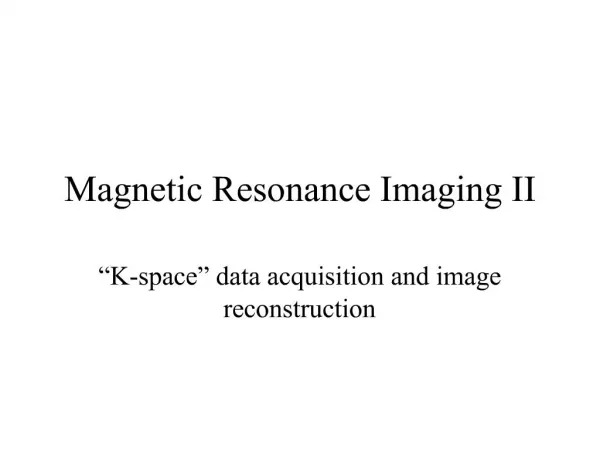
Magnetic Resonance Imaging II
420 likes | 725 Vues
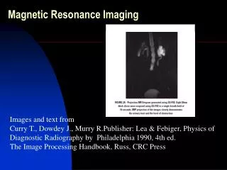
K-space matrix. MR data are initially stored in the k-space matrix, the frequency domain" repositoryThe axes have units of cycles/unit distanceEach axis is symmetric about the center of k-space, ranging from fmax to fmaxLow-frequency signals are mapped around the origin of k-space and high-fre

Magnetic Resonance Imaging II
E N D
Presentation Transcript
1. Magnetic Resonance Imaging II �K-space� data acquisition and image reconstruction
2. K-space matrix MR data are initially stored in the k-space matrix, the �frequency domain� repository
The axes have units of cycles/unit distance
Each axis is symmetric about the center of k-space, ranging from �fmax to +fmax
Low-frequency signals are mapped around the origin of k-space and high-frequency signals are mapped further from the origin in the periphery
4. K-space matrix (cont.) Frequency domain data are encoded in the kx direction by the frequency encode gradient (FEG), and in the ky direction by the phase encode gradient (PEG) in most image sequences
Lowest spatial frequency increment is the bandwidth across each pixel
6. Two-dimensional data acquisition MR data acquired as a complex, composite frequency waveform
With methodical variations of the PEG during each acquisition, the k-space matrix is filled to produce the desired variations across the frequency and phase encode directions
8. Narrow band RF excitation pulse applied simultaneously with the slice select gradient (SSG)
Energy absorption dependent on amplitude and duration of the RF pulse at resonance
Longitudinal magnetization converted to transverse magnetization, extent of which depends on saturation of spins and angle of excitation
90-degree flip angle produces maximal transverse magnetization
10. Phase encode gradient (PEG) applied for a brief duration to create phase difference among spins along the phase encode direction
Produces several �views� of the data along the ky axis, corresponding to the strength of the PEG
Refocusing 180-degree pulse delivered after selectable delay time, TE/2
Inverts direction of individual spins and reestablishes phase coherence of transverse magnetization with formation of echo at time TE
12. During echo formation and subsequent decay, frequency encode gradient (FEG) applied orthogonal to both slice select and phase encode gradient directions
Encodes precessional frequencies spatially along the readout gradient
14. Simultaneous to application of FEG and echo formation, computer acquires the time-domain signal using an analog-to-digital converter (ADC)
Sampling rate determined by excitation bandwidth
One-dimensional Fourier transform converts the digital data into discrete frequency values and corresponding amplitudes
Proton precessional frequencies determine position along the kx (readout) direction
16. Data deposited in k-space matrix in a row, specifically determined by the PEG strength applied during excitation
Incremental variation of the PEG throughout the acquisition fills the matrix one row at a time
Possible to acquire the phase encode data in nonsequential order to fill portions of k-space more pertinent to the requirements of the exam (e.g., in low-frequency, central area of k-space)
After matrix is filled, columns contain positionally dependent phase change variations along the ky (phase encode) direction
18. Two-dimensional inverse Fourier transform decodes the frequency domain information piecewise along the rows and then along the columns of k-space
Final image is a spatial representation of the proton density, T1, T2, and flow characteristics of the tissue using a gray-scale range
Each pixel represents a voxel; thickness determined by slice select gradient strength and RF frequency bandwidth
19. K-space segmentation Central area of k-space (lower spatial frequencies) represents the bulk of the anatomical information
Information near the center of k-space provides the large area contrast in the image
Outer areas in k-space contribute to the resolution and detail
21. 2D multiplanar acquisition Direct axial, coronal, sagittal, or oblique planes can be obtained by energizing the appropriate gradient coils during image acquisition
The slice select gradient determines the orientation of the slices
Axial uses the z-axis coils
Coronal uses the y-axis coils
Sagittal uses the x-axis coils
Oblique plane acquisition depends on a combination of two or more coils energized simultaneously
23. Acquisition time Time required to acquire an image is equal to
Spin echo sequence for a 256 x 192 image matrix and two averages per phase encode step with TR = 600 msec yeilds an imaging time of 3.84 minutes
Where nonsquare pixels are used, the phase encode direction is typically placed along the small dimension of the image matrix
24. Multislice data acquisition Average time per slice significantly reduced using multiple slice acquisition methods
Several slices within the tissue volume selectively excited during a TR interval to fully utilize the (dead) time waiting for longitudinal recovery in a specific slice
This requires cycling all of the gradients and tuning the RF excitation pulse many times during the TR interval
26. Multislice data acquisition (cont.) Total number of slices is a function of TR, TE, and machine limitations:
C is a constant dependent on MR equipment capabilities (computer speed, gradient capabilities, RF cycling, etc.)
Long TR acquisitions such as proton density and T2-weighted sequences provide greater number of slices than T1-weighted sequences with short TR
27. Data synthesis Data �synthesis� takes advantage of the symmetry and redundant characteristics of the frequency domain signals in k-space
Acquistion of as little as one-half the data plus one row of k-space allows the mirroring of �complex conjugate� data to fill the remainder of the matrix
Reduces the acquisition time by nearly one-half
Penalty is a reduction in the SNR and potential for artifacts
29. Fast spin echo acquisition FSE technique uses multiple phase encode steps in conjunction with multiple 180-degree refocusing RF pulses per TR interval to produce a train of up to 16 echoes
Each echo experiences differing amounts of phase encoding that correspond to different lines in k-space
Points near the center of k-space acquired from first echoes for best SNR
31. Inversion recovery acquisition Phase and frequency encoding occur similarly to the spin echo pulse sequence
Since TR is typically long, several slices can be acquired within the volume of interest
STIR (short tau inversion recovery) and FLAIR (fluid attenuated inversion recovery) pulse sequences are commonly used
33. Gradient recalled echo acquisition Similar to standard spin echo sequence with a readout gradient reversal substituting for the 180-degree pulse
With small flip angles and gradient reversals, considerable reduction in TR and TE is possible for fast image acquistion; ability to acquire multiple slices is compromised
PEG rewinder pulse of opposite polarity applied to maintain phase relationship from pulse to pulse
35. GRE acquisition (cont.) Gradient echo image acquisition time given by same expression as for spin echo technique
Gradient-echo sequence for a 256 x 192 image matrix, two averages, and TR = 30 msec, imaging time is approximately 15.5 seconds
Compromises include SNR losses, magnetic susceptibility artifacts, and less immunity from magnetic field inhomogeneities
36. Echo planar image acquistion EPI acquisition provides extremely fast imaging time
For single-shot EPI, image acquisition typically begins with a standard 90-degree flip, then a PEG/FEG gradient application to initiate acquisition of data in periphery of k-space, followed by a 180-degree echo-producing pulse
Immediately after, an oscillating readout gradient and phase encode gradient �blips� are continuously applied to stimulate echo formation and rapidly fill k-space in a stepped pattern
38. EPI acquistion (cont.) Echo planar images typically have poor SNR, low resolution, and many artifacts
Technique offers real-time �snapshot� image capability with 50 msec or less total acquisition time
Emerging as a clinical tool for studying time-dependent physiologic processes and functional imaging
39. My brain� hurts
With apologies to Monty Python