Particle Physics

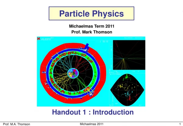
Particle Physics Michaelmas Term 2011 Prof Mark Thomson g X g g X g Handout 3 : Interaction by Particle Exchange and QED Michaelmas 2011

m+ e+ g m– e– e– e– |M|2 x (phase space) s  flux q q Recap • Working towards a proper calculation of decay and scattering processes lnitially concentrate on: • e+e–  m+m– • e– q  e– q • In Handout 1 covered the relativistic calculation of particle decay rates and cross sections • In Handout 2 covered relativistic treatment of spin-half particles Dirac Equation • This handout concentrate on the Lorentz Invariant Matrix Element • Interaction by particle exchange • Introduction to Feynman diagrams • The Feynman rules for QED Michaelmas 2011

f j i i Interaction by Particle Exchange • Calculate transition rates from Fermi’s Golden Rule where is perturbation expansion for the Transition Matrix Element • For particle scattering, the first two terms in the perturbation series • can be viewed as: f “scattering in a potential” “scattering via an intermediate state” • “Classical picture”– particles act as sources for fields which give • rise a potential in which other particles scatter –“action at a distance” • “Quantum Field Theory picture”– forces arise due to the exchange • ofvirtual particles. No action at a distance + forces between particles • now due to particles Michaelmas 2011

Consider the particle interaction which occurs • via an intermediate state corresponding to the exchange of particle c a Initial state i : Vji space Final state f : x Intermediate state j : • This time-ordered diagram corresponds to • a“emitting”x and then b absorbing x Vfj b d f i j time • refers to the time-ordering where aemits x before b absorbs it (start of non-examinable section) • One possible space-time picture of this process is: • The corresponding term in the perturbation expansion is: Michaelmas 2011

Need an expression for in non-invariant matrix element • Ultimately aiming to obtain Lorentz Invariant ME is related to the invariant matrix element by • Recall c a ga x is the “Lorentz Invariant” matrix element for a c + x is a measure of the strength of the interaction a c + x where k runs over all particles in the matrix element • Here we have • The simplest Lorentz Invariant quantity is a scalar, in this case Note : the matrix element is only LI in the sense that it is defined in terms of LI wave-function normalisations and that the form of the coupling is LI Note : in this “illustrative” example g is not dimensionless. Michaelmas 2011

Similarly x gb b d Giving • The “Lorentz Invariant” matrix element for the entire process is Note: • refers to the time-ordering where a emits x before b absorbs it It is not Lorentz invariant, order of events in time depends on frame • Momentum is conserved at each interaction vertex but not energy • Particle xis “on-mass shell” i.e. Michaelmas 2011

c a • This time-ordered diagram corresponds to • b“emitting”x and then a absorbing x space ~ ~ ~ • x is the anti-particle of x e.g. b d ne ne e– e– f i j W+ W– time nm nm m– m– Energy conservation: • But need to consider also the other time ordering for the process • The Lorentz invariant matrix element for this time ordering is: • In QM need to sum over matrix elements corresponding to same final state: Michaelmas 2011

After summing over all possible time orderings, is (as anticipated) • Lorentz invariant.This is a remarkable result – the sum over all time • orderings gives a frame independent matrix element. • Which gives • From 1st time ordering c a ga giving (end of non-examinable section) • Exactly the same result would have been obtained by considering the • annihilation process Michaelmas 2011

c c c a a a space space • The factor is the propagator; it arises naturally from • the above discussion of interaction by particle exchange d d b b b d time time c a b d Feynman Diagrams • The sum over all possible time-orderings is represented by a • FEYNMAN diagram • In a Feynman diagram: • the LHS represents the initial state • the RHS is the final state • everything in between is “how the interaction • happened” • It is important to remember that energy and momentum are conserved • at each interaction vertex in the diagram. Michaelmas 2011

For elastic scattering: c a b d • The matrix element: depends on: • The fundamental strength of the interaction at the two vertices • The four-momentum, , carried by the (virtual) particle which is • determined from energy/momentum conservation at the vertices. • Note can be either positive or negative. Here “t-channel” q2 < 0 termed “space-like” Here “s-channel” In CoM: q2 > 0 termed “time-like” Michaelmas 2011

a c a c a c space space b b d d d b time time Virtual Particles Feynman diagram “Time-ordered QM” • Momentum AND energy conserved • at interaction vertices • Exchanged particle “off mass shell” • Momentum conserved at vertices • Energy not conserved at vertices • Exchanged particle “on mass shell” VIRTUAL PARTICLE • Can think of observable “on mass shell” particles as propagating waves • and unobservable virtual particles as normal modes between the source • particles: Michaelmas 2011

c a b d f i p V(r) • In this way can relate potential and forces to the particle exchange picture • However, scattering from a fixed potential is not a relativistic invariant view Aside: V(r) from Particle Exchange • Can view the scattering of an electron by a proton at rest in two ways: • Interaction by particle exchange in 2nd order perturbation theory. • Could also evaluate the same process in first order perturbation • theory treating proton as a fixed source of a field which gives • rise to a potential V(r) Obtain same expression for using YUKAWA potential Michaelmas 2011

(here charge) Quantum Electrodynamics (QED) • Now consider the interaction of an electron and tau lepton by the exchange of a photon. Although the general ideas we applied previously still hold, we now have to account for the spinof the electron/tau-lepton and also the spin (polarization) of the virtual photon. (Non-examinable) • The basic interaction between a photon and a charged particle can be • introduced by making the minimal substitution (part II electrodynamics) In QM: Therefore make substitution: where • The Dirac equation: Michaelmas 2011

Potential energy Combined rest mass + K.E. • We can identify the potential energy of a charged spin-half particle • in an electromagnetic field as: (note the A0 term is just: ) • The final complication is that we have to account for the photon • polarization states. e.g. for a real photon propagating in the z direction we have two orthogonal transverse polarization states Could equally have chosen circularly polarized states Michaelmas 2011

e– e– • In QED we could again go through the procedure of summing the time-orderings using Dirac spinors and the expression for . If we were to do this, remembering to sum over all photon polarizations, we would obtain: t– t– • Previously with the example of a simple spin-less interaction we had: a c = = ga gb d b Interaction of t– with photon Massless photon propagator summing over polarizations Interaction of e– with photon • All the physics of QED is in the above expression ! Michaelmas 2011

The sum over the polarizations of the VIRTUAL photon has to include • longitudinal and scalar contributions, i.e. 4 polarisation states This is not obvious – for the moment just take it on trust and gives: and the invariant matrix element becomes: (end of non-examinable section) • Using the definition of the adjoint spinor • This is a remarkably simple expression ! It is shown in Appendix V of Handout 2 that transforms as a four vector. Writing showing that M is Lorentz Invariant Michaelmas 2011

m+ e+ g m– e– Feynman Rules for QED • It should be remembered that the expression hides a lot of complexity. We have summed over all possible time- orderings and summed over all polarization states of the virtual photon. If we are then presented with a new Feynman diagram we don’t want to go through the full calculation again. Fortunately this isn’t necessary – can just write down matrix element using a set of simple rules Basic Feynman Rules: • Propagator factor for each internal line (i.e. each internal virtual particle) • Dirac Spinor for each external line (i.e. each real incoming or outgoing particle) • Vertex factor for each vertex Michaelmas 2011

External Lines incoming particle outgoing particle spin 1/2 incoming antiparticle outgoing antiparticle incoming photon spin 1 outgoing photon • Internal Lines (propagators) n m spin 1 photon spin 1/2 fermion • Vertex Factors spin 1/2 fermion (charge -|e|) • Matrix Element = product of all factors Basic Rules for QED Michaelmas 2011

e– e– t– t– m+ e.g. e+ g m– e– • At each vertex the adjoint spinor is written first • Each vertex has a different index • The of the propagator connects the indices at the vertices e.g. e– e– t– t– • Which is the same expression as we obtained previously Note: Michaelmas 2011

Summary • Interaction by particle exchange naturally gives rise to Lorentz Invariant Matrix Element of the form • Derived the basic interaction in QED taking into account the spins of the fermions and polarization of the virtual photons: • We now have all the elements to perform proper calculations in QED ! Michaelmas 2011

Particle Physics