Lecture 31. Controllability
Lecture 31. Controllability. The general idea of control. The algebraic controllability theorem. How to control a linear SISO system to zero: the fundamentals of feedback control. We have a general picture that I put in for completeness only.

Lecture 31. Controllability
E N D
Presentation Transcript
Lecture 31. Controllability The general idea of control The algebraic controllability theorem How to control a linear SISO system to zero: the fundamentals of feedback control
We have a general picture that I put in for completeness only We know that (linear) dynamics can be modeled by We want to make some subset or combination of the states to do something we want. We call this the output These equations are for the general multi-input, multi-output case
We are generally going to restrict ourselves to linear single input-single output (SISO) systems scalars Denote the dimension of the state vector by N Then A is a N x N matrix b a Nx 1 (column) vector cT a I xN (row) vector N denotes the dimension of the state, NOT the number of degrees of freedom
We want to make y do what we want. This has some implications for what x does For now, let me focus on x and not worry about y — If I can make x do what I want, ywill be easy Denote the desired behavior of x by xd, the error then I can write what we want
Write the differential equation in terms of the desired response and the error where I have allowed for the possibility that the desired response requires an input Split the equations (they’re linear, so that’s not an issue) The idea is to find ud — we’ll work on this another time open loop control closed loop correction This is the fundamental error dynamics equation: we want x to go to 0
We’re going to start with xd = 0 so I can avoid having to find ud We will eventually (given “worlds enough and time”) look at tracking I don’t need the subscript, so I’ll stop writing it for now The control problem for now is: given find u as a function of x such that x —> 0 Is it possible to solve the problem?! Closed loop correction from slide 6 BTW. If the problem is stable, then we don’t need control to make x go to 0.
We know how to find xgiven u We simply find the state transition matrix and apply the formulas But that may be easier said than done; there are other things we can do. It also doesn’t tell us how to find u to make x go to zero
We saw last time that there are situations where the input cannot reach all the states (eigenvectors/eigenfunctions) The sense of this is not always clear If any of the elements of z is not connected to u, that element cannot be controlled This may or may not be an actual problem — more on that anon We need a criterion whereby we can tell if a system is controllable It should be based on A and B, so that we can figure this out before wasting too much time But first
Stability for any problem NB. I have used s here I have used l elsewhere They are equivalent Both are eigenvalues Both have an associated eigenvector there will be a homogeneous solution which we can write Suppose s ≠ 0: If Re(si) < 0 for alli the homogeneous solution will decay in time We call this (asymptotically) stable If Re(si) > 0 for anyi the homogeneous solution will grow in time We call this (linearly) unstable If Re(si) = 0 for alli the homogeneous solution will oscillate in time We call this marginally stable
If s = 0 we have algebraic eigenfunctions. We’ll be dealing with these as special cases. Stability is important because in real life there will always be some tiny part of the homogeneous solution in the answer If the solution contains an unstable part, it will grow without bound, and the uncontrolled system will “blow up” We need controls to prevent this Let’s suppose that we need or want control and return to the question IS CONTROL POSSIBLE?
The algebraic controllability theorem For a general linear system (including multi-input systems) The controllability matrix is The system is controllable if and only if the rank of Q = N The theorem is true for multi-input systems
What do these matrices look like? What am I doing here? Let’s look at a four dimensional two input system symbolically
The matrix Q will be square, NxN, for a single input system If there are M inputs then Q has N rows and MNcolumns as in the symbolic example we just saw: N = 4, M = 2, MN = 8 An NxN matrix has rank Niff its determinant is nonzero, so the rank criterion works for square and nonsquare matrices Let’s look at a simple example to see how this goes
u and we can draw a block diagram of this x3 -3 x2 x1 + u - -2 -1
How did I do that? u x3 -3 x2 x1 + u - -2 -1
How did I do that? The diagonal terms of A u x3 -3 x2 x1 + u - -2 -1
How did I do that? The off-diagonal terms of A u x3 -3 x2 x1 + u - -2 -1
Now let’s carry on and find Q We’ll see the procedure I went through in the general 4, 2 case
You can find the rank by row reduction (or ask Mathematica) or find the determinant (expanding by minors)
So, what happens next? Not only does this give us a controllability test, but it starts us on the road to putting the basic problem in companion form We want to modify A and b, and we do this using another TAT-1 transformation But, what is T? It is NOT the same T that we used to diagonalize and this is NOT the same z state
We start with Q (and restrict ourselves to SI systems) This is a set of columns, as we have seen before Q is invertible, because its determinant is not zero. Take the last row of Q-1 This is the first row of T, and we build the whole T on the next slide
and then the z equations follow the same way as before This is not the same z as that we found diagonalizing
This can be done by hand, but is a little messy and lot tedious, so . . .
We can finally apply the differential equation in transformed form Of course, the eigenvalues of A1 are the same as those of A
This is not the same z as the z that we used in the diagonalization exercises and we have a nice block diagram for this + z1 u - -6 -11 -6
The old block diagram u x3 -3 x2 x1 + u - -2 -1
It is interesting note that the transfer function approach would give us the same dynamics I think I will leave that for you to establish. Let’s revisit the diagonalizing transformation for this case
What do we need to do? We need the matrix of the eigenvectors, V = T-1 We need its inverse, V-1 = T The new matrix is diagonal with its nonzero elements equal to the eigenvalues of A Summarize on the next slide
u -3 u -2 u -1
So we have three different pictures corresponding to the same dynamics
Original problem u x3 -3 x2 x1 + u - -2 -1
Companion (phase canonical) form + z1 u - -6 -11 -6
u Diagonalized form -3 u -2 u -1
Let’s get back to thinking about the companion form dynamics The eigenvalues are -3, -2, and -1 The characteristic polynomial must be
Consider another three dimensional system, this one unstable, so we are more motivated to find a control Diagonalization The eigenvalues of A are -2, -1 and +1 The matrix of the eigenvectors is
Its inverse is T so we have Tb which suggest that this a controllable system
u Its block diagram -2 u -1 the eigenvalues u from Tb the unstable part 1
We can go through the controllability theorem for this one The determinant is +6, so it is invertible and the system is controllable Now we can move on to find the companion form of A and b
So that companion form Once we have found z, we need to get x back!
Now let’s reflect on the control aspects of this problem Suppose we want x to go to zero. xwill go to zero if z goes to zero That is easier to do than working directly with the x formulation. The system is unstable because we have a positive eigenvalue We have the transformed problem in z space How can we move the eigenvalues from unstable to stable?
The bottom row of A1 contains the coefficients of the characteristic polynomial for the uncontrolled, open loop, homogeneous system