Lecture 3 Tuesday, 2/9/10 Amortized Analysis
250 likes | 502 Vues
UMass Lowell Computer Science 91.503 Graduate Analysis of Algorithms Prof. Karen Daniels Spring, 2010. Lecture 3 Tuesday, 2/9/10 Amortized Analysis. Overview. Amortize: “To pay off a debt, usually by periodic payments” [ Websters ] Amortized Analysis: “creative accounting” for operations

Lecture 3 Tuesday, 2/9/10 Amortized Analysis
E N D
Presentation Transcript
UMass Lowell Computer Science 91.503GraduateAnalysis of AlgorithmsProf. Karen DanielsSpring, 2010 Lecture 3 Tuesday, 2/9/10 Amortized Analysis
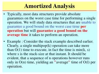
Overview • Amortize: “To pay off a debt, usually by periodic payments” [Websters] • Amortized Analysis: • “creative accounting” for operations • can show average cost of an operation is small (when averaged over sequence of operations, not distribution of inputs) even though a single operation in the sequence is expensive • result must hold for any sequence of these operations • no probability is involved (unlike average-case analysis) • guarantee holds in worst-case • analysis method only; no effect on code operation
Overview (continued) • 3 ways to determine amortized cost of an operation that is part of a sequence of operations: • Aggregate Method • find upper bound T(n) on total cost of sequence of n operations • amortized cost = average cost per operation = T(n)/n • same for all the operations in the sequence • Accounting Method • amortized cost can differ across operations • overcharge some operations early in sequence • store overcharge as “prepaid credit” on specific data structure objects • Potential Method • amortized cost can differ across operations (as in accounting method) • overcharge some operations early in sequence (as in accounting method) • store overcharge as “potential energy” of data structure as a whole • (unlike accounting method)
Aggregate Method:Stack Operations see example • Aggregate Method • find upper bound T(n) on total cost of sequence of n operations • amortized cost = average cost per operation = T(n)/n • same for all the operations in the sequence • Traditional Stack Operations • PUSH(S,x) pushes object x onto stack S • POP(S) pops top of stack S, returns popped object • O(1) time: consider cost as 1 for our discussion • Total actual cost of sequence of n PUSH/POP operations = n • STACK-EMPTY(S) time in Q(1)
MULTIPOP(S,k) 1 while not STACK-EMPTY(S) and k = 0 2 do POP(S) 3 k k - 1 Aggregate Method:Stack Operations (continued) • New Stack Operation • MULTIPOP(S,k) pops top k elements off stack S • pops entire stack if it has < k items • MULTIPOP actual cost for stack containing s items: • Use cost =1 for each POP • Cost = min(s,k) • Worst-case cost in O(s) in O(n)
Aggregate Method:Stack Operations (continued) • Sequence of n PUSH, POP, MULTIPOP ops • initially empty stack • MULTIPOP worst-case O(n) O(n2) for sequence • Aggregate method yields tighter upper bound • Sequence of n operations has O(n) worst-case cost • Each item can be popped at most once for each push • # POP calls (including ones in MULTIPOP) <= #push calls • <= n • Average cost of an operation = O(n)/n = O(1) • = amortized cost of each operation • holds for PUSH, POP and MULTIPOP
Accounting Method stay out of debt! • Accounting Method • amortized cost can differ across operations • overcharge some operations early in sequence • store overcharge as “prepaid credit” on specific data structure objects • Let be actual cost of ith operation • Let be amortizedcost of ith operation (what we charge) • Total amortized cost of sequence of operations must be upper bound on total actual cost of sequence • Total credit in data structure = • must be nonnegativefor all n
Actual Cost Operation Assigned Amortized Cost • PUSH 1 2 • POP 1 0 • MULTIPOP min(k,s) 0 Accounting Method:Stack Operations • Paying for a sequence using amortized cost: • start with empty stack • PUSH of an item always precedes POP, MULTIPOP • pay for PUSH & store 1 unit of credit • credit for each item pays for actual POP, MULTIPOP cost of that item • credit never “goes negative” • total amortized cost of any sequence of n ops is in O(n) • amortized cost is upper bound on total actual cost see example
terms telescope Potential Method • Potential Method • amortized cost can differ across operations (as in accounting method) • overcharge some operations early in sequence (as in accounting method) • store overcharge as “potential energy” of data structure as a whole (unlike accounting method) • Let ci be actual cost of ith operation • Let Di be data structure after applying ith operation • Let F(Di ) be potential associated with Di • Amortized cost of ith operation: • Total amortized cost of n operations: • Require: so total amortized cost is upper bound on total actual cost • Since n might not be known in advance, guarantee “payment in advance” by requiring
Potential Method:Stack Operations • Potential function value = number of items in stack • guarantees nonnegative potential after ith operation • Amortized operation costs (assuming stack has s items) • PUSH: • potential difference= • amortized cost = • MULTIPOP(S,k) pops k’=min(k,s) items off stack • potential difference= • amortized cost = • POP amortized cost also = 0 • Amortized cost O(1) total amortized cost of sequence of n operations in O(n) see example
Dynamic Tables:Overview • Dynamic Table T: • array of slots • Ignore implementation choices: stack, heap, hash table... • if too full, increase size & copy entries to T’ • if too empty, decrease size & copy entries to T’ • Analyze dynamic table insert and delete • Actual expansion or contraction cost is large • Show amortized cost of insert or delete in O(1) • Load factor a(T) = num[T]/size[T] • empty table: a(T) = 1 (convention guaranteeing load factor can be lower bounded by a useful constant) • full table: a(T) = 1
Dynamic Tables:Table (Expansion Only) • Load factor bounds (double size when T is full): • Sequence of n inserts on initially empty table • Worst-case cost of insert is in O(n) • Worst-case cost of sequence of n inserts is in O(n2) WHY? LOOSE “elementary” insertion Double only when table is already full.
Dynamic Tables:Table Expansion (cont.) Amortized Analysis see example • Aggregate Method: • ci= i if i-1 is exact power of 2 • 1 otherwise • total cost of n inserts = count only elementary insertions Accounting Method: • charge cost = 3 for each element inserted • intuition for 3 • each item pays for 3 elementary insertions • inserting itself into current table • expansion: moving itself • expansion: moving another item that has already been moved
Dynamic Tables:Table Expansion (cont.) Amortized Analysis • Potential Method: • Value of potential function F(T) • 0 right after expansion (then becomes 2) • builds to table size by time table is full • always nonnegative, so sum of amortized costs of n inserts is upper bound on sum of actual costs • Amortized cost of ith insert • Fi= potential after ith operation • Case 1: insert does not cause expansion • Case 2: insert causes expansion 3 functions: sizei, numi, Fi use these:
Dynamic Tables:Table Expansion & Contraction count elementary insertions & deletions • Load factor bounds: • (double size when T is full) (halve size when T is ¼ full): • DELETE pseudocode analogous to INSERT same as INSERT Amortized Analysis • Potential Method: • Value of potential function F(T) • = 0 for empty table • 0 right after expansion or contraction • builds as a(T) increases to 1 or decreases to ¼ • always nonnegative, so sum of amortized costs of n inserts is upper bound on sum of actual costs • = 0 when a(T)=1/2 • = num[T] when a(T)=1 • = num[T] when a(T)=1/4
Dynamic Tables:Table Expansion & Contraction Amortized Analysis Potential Method
Dynamic Tables:Table Expansion & Contraction Amortized Analysis Potential Method • Analyze cost of sequence of n inserts and/or deletes • Amortized cost of ith operation • Case 1: INSERT • Case 1a: ai-1 >= ½. By previous insert analysis: • Case 1b: ai-1 < ½ and ai < ½ • Case 1c: ai-1 < ½ and ai >= ½ holds whether or not table expands no expansion no expansion see derivation in textbook
Dynamic Tables:Table Expansion & Contraction Amortized Analysis Potential Method • Amortized cost of ith operation (continued) • Case 2: DELETE • Case 2a: ai-1 >= ½. • Case 2b: ai-1 < ½ and ai < ½ • Case 2c: ai-1 < ½ and ai < ½ textbook exercise no contraction contraction Conclusion: amortized cost of each operation is bounded above by a constant, so time for sequence of n operations is O(n).
Example: Dynamic Closest Pair S S S source: “Fast hierarchical clustering and other applications of dynamic closest pairs,” David Eppstein, Journal of Experimental Algorithmics, Vol. 5, August 2000.
Example: Dynamic Closest Pair (continued) S S S source: “Fast hierarchical clustering and other applications of dynamic closest pairs,” David Eppstein, Journal of Experimental Algorithmics, Vol. 5, August 2000.
Example: Dynamic Closest Pair (continued) Rules • Partition dynamic set S into subsets. • Each subset Si has an associated digraph Gi consisting of a set of disjoint, directed paths. • Total number of edges in all graphs remains linear • Combine and rebuild if number of edges reaches 2n. • Closest pair is always in some Gi. • Initially all points are in single set S1. • Operations: • Create Gi for a subset Si. • Insert a point. • Delete a point. • Merge subsets until . We use log base 2. source: “Fast hierarchical clustering and other applications of dynamic closest pairs,” David Eppstein, Journal of Experimental Algorithmics, Vol. 5, August 2000.
Example: Dynamic Closest Pair (continued) Rules: Operations source: “Fast hierarchical clustering and other applications of dynamic closest pairs,” David Eppstein, Journal of Experimental Algorithmics, Vol. 5, August 2000. • Create Gi for a subset Si: • Select starting point (we choose leftmost (or higher one in case of a tie)) • Iteratively extend the path P, selecting next vertex as: • Case 1: nearest neighbor in S \ P if last point on path belongs to Si • Case 2: nearest neighbor in Si \ P if last point on path belongs to S\Si • Insert a point x: • Create new subset Sk+1={x}. • Merge subsets if necessary. • Create Gifor new or merged subsets. • Delete a point x: • Create new subset Sk+1= all points y such that (y,x) is a directed edge in some Gi. • Remove x and adjacent edges from all Gi. (We also remove y from its subset.) • Merge subsets if necessary. • Create Gifor new or merged subsets. • Merge subsets until : • Choose subsets Siand Sjto minimize size ratio |Sj|/ |Si|. See handout for example.
Example: Dynamic Closest Pair (continued) Potential Function source: “Fast hierarchical clustering and other applications of dynamic closest pairs,” David Eppstein, Journal of Experimental Algorithmics, Vol. 5, August 2000. • Potential for a subset Si : Fi = n|Si|log|Si|. • Total potential F = n2logn - SFi. • Paper proves this Theorem: • HW#3 presents variation on these operations and asks you to determine the amortized cost per insertion and deletion. Theorem: The data structure maintains the closest pair in S in O(n) space, amortized time O(nlogn) per insertion, and amortized time O(nlog2n)per deletion.
