Understanding Amortized Analysis of Data Structure Operations
This text explores amortized analysis, a technique used to evaluate the average performance of data structure operations over time rather than focusing solely on the worst-case scenario for a single operation. It explains how sequences of operations can result in an average cost of operation lower than the worst-case cost. The document outlines methods such as the aggregate method, accounting method, and potential method, providing examples like a two-stack system to illustrate how these approaches manage and analyze operation costs to ensure efficiency.

Understanding Amortized Analysis of Data Structure Operations
E N D
Presentation Transcript
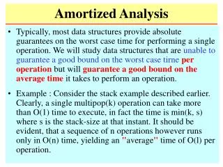
Amortized Analysis • Typically, most data structures provide absolute guarantees on the worst case time for performing a single operation. We will study data structures that are unable to guarantee a good bound on the worst case tirneper operation but will guarantee a good bound on the average time it takes to perform an operation. • Example : Consider the stack example described earlier. Clearly, a single multipop(k) operation can take more than O(1) time to execute, in fact the time is min(k, s) where s is the stack-size at that instant. It should be evident, that a sequence of n operations however runs only in O(n) time, yielding an "average" time of O(l) per operation.
Amortized Analysis • In an amortized analysis the time required to perform a sequence of data structure operations is averaged over all the operations performed. • Amortized analysis can be used to show that the average cost of an operation is small, if one averages over a sequence of operations, even though a single operation might be expensive. • Amortized analysis differs from average case analysis in that probability is not involved; an amortized analysisguarantees the average performance of each operation in the worst case.
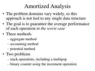
Formal Schemes for Amortized Analysis • Aggregate method. • Accounting method. • Potential method.
The Aggregate Method • Evaluate the overall worst-case cost T(n) (an upper bound) on the total cost of a sequence of n operations. • In the worst case, the average cost, or amortized cost, per operation is therefore T(n)/n. • Note that the amortized cost for any operation is the same in the aggregate method. On the contrary, the accounting method and the potential method, may assign different amortized costs to different types of operations. • Note that T(n)/n is not an average complexity measure in the sense of averaging over lots of different possible inputs. It is a worst-case measure, but expressed in cost per operation.
Example: Two-Stack System • Suppose there are two stacks called A and B, manipulated by the following operations: • push(S, d): Push a datum d onto stack S. Real Cost = 1. • multi-pop(S, k): Removes min(k, |S|) elements from stack S. Real Cost = min(k, |S|). • transfer(k): Repeatedly pop elements from stack A and push them onto stack B. until either k elements have been moved, or A is empty. Real Cost = # of elements moved = min(k, |A|).
n push operations n elements popped • n elements transferred Illustration B A
Aggregate Method • For a sequence of n operations, there are ≤ n data pushed into either A or B. Therefore there are ≤ n data popped out from either A or B and ≤ n data transferred from A to B. Thus, the total cost of the n operations is ≤ 3n. Thus.
The Accounting Method • Assign fixed (possibly different) coststo operations. Compute the aggregate cost based on the fixed costs. • There are operations that are overpaidas well as those that are underpaid. • The accounting method overcharges some operations early in the sequence, storing the overcharge as "prepaid credit" on specific objects in the data structure. • The credit is used later in the sequence to pay for operations that are charged less than they actually cost. • Argue that the total underpayment does not exceed the total overpayment.
Push(A,d) Pop(A,d) Pop(B,d) Transferred() Illustration B A
Accounting Method • push(A, d): $3 -- This pays for the push and a pop of the push a transfer and a pop. • push(B, d): $2 -- This pays for the push and a pop. • multi-pop(S, k): $0 • transfer(k): $0 • After any n operations you will have 2|A| + |B| dollars in the bank. Thus the bank account never goes negative. Furthermore the amortized cost of the n operations is O(n) (more precisely ≤ 3n).
The Potential Method • D0: the initial data structure on which n operations are performed. • Di: the data structure that results after applying the ith operation to data structure Di-1. • ci: the actual cost of the ith operation • F: a potential function maps each data structure Di to a real number F(Di), which is the potential associated with data structure Di. • ĉi: the amortized cost of the ith operation w.r.t. F ĉi = ci + F(Di) - F(Di-1) = ci + DF ĉi = [ci + F(Di) - F(Di-1)] = ci + F(Di) - F(Di-1)
Illustration c1 c2 c3 c4 cn D0 D1 D2 D3 … Dn ĉ1 ĉ2 ĉ3 ĉ4ĉn F(D0) F(D1) F(D2) F(D3) …
Potential Function Method • Let F(A, B) = 2|A| + |B|, then • ĉ(push(A, d)) = 1 + DF = 1 + 2 = 3 • ĉ(push(B, d)) = 1 + DF = 1 + 1 = 2 • ĉ(multi-pop(A, k)) = min(k, |A|) + DF = -min(k, |A|) • ĉ(multi-pop(B, k)) = min(k, |B|) + DF = 0 • ĉ(transfer(k)) = min(k, |A|) + DF =0 Σĉ = Σc + DF Σc = Σĉ - DF ≤ Σĉ≤ 3n = O(n). • If we can pick F so that F(Di) F(D0) for all i, and that Σĉ is easy to compute, then Σĉ/n upper-bounds the average cost.
Incrementing a k-bit Counter • Incrementing a k-bit nary counter n times starting from 0. Is the cost of increment O(k)? • Aggregate Method: The i-th bit is flipped only at every 2i-1th step. So the total number of bit flips is • Accounting Method: Set the cost of setting (resetting) a bit to 2 (0). Since a bit cannot be reset unless it is set, the total underpayment is at most the total overpayment. • Potential Method: Define F(Di) to be bi, the number of bits 1 in the counter. Let ti be the number of bits that are reset at the ith operation. Then ci = ti +1and ĉ = ti +1+ DF = ti +1+ (1 - ti) = 2. So, the total amortized cost is at most 2n.
Dynamic Tables • A dynamic table is a table of variable size, where an expansion (or a contraction is caused when the load factor has become larger (or smaller) than a fixed threshold. • Let the expansion threshold be 1 and the expansion rate be 2; i.e., the table size is doubled when an item is to be inserted when the table is full. • Let the contraction threshold be 1/4 and the contraction rate be 1/2; i.e., the table size is halved when an item is to be eliminated when the table is exactly one-fourth full.
Implementation of Expansion/Contraction • When one of these operations take place we create a new table and move all the elements from the old one to the new one. • Suppose that there are n calls of insertion/deletion made, what is the average cost of each operation (in the worst case)?
Expansion/Contraction • If the size is kept the same the cost is O(1). • If the size is doubled from M to 2M, the actual cost is M+1. The next table size change is after at least M steps for doubling and at least M/2 steps for halving. So the actual cost can be spread over the next M/2 “normal" steps to yield an amortized cost of O(1). • If the size is halved from M to M/2, the actual cost is M/4. The next table size change is after at least 3M/4 steps for doubling and at least M/8 steps for halving. So the actual cost can be spread over the next M/8 steps to yield an amortized cost of O(1).