Amortized Analysis
Explore amortized analysis techniques for assessing time complexity, including the aggregate, accounting, and potential methods. Learn how these methods can provide a more accurate understanding of the cost of sequences of operations, such as push, pop, and multipop in dynamic arrays and binary counters.

Amortized Analysis
E N D
Presentation Transcript
Problem • What is the time complexity of n insert operations into an dynamic array, which doubles its size each time it is completely filled. • for (int i=0; i<n; i++) { insert (i) // O(n) }
Problem • Until now we analyzed the execution time of such loop as , but not all insert operation do indeed take O(n) • We try to find a tighter bound for the execution time of a series of n insert operations
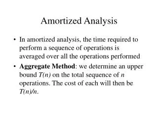
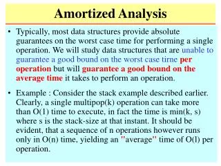
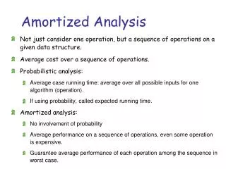
Amortized Analysis techniques • In amortized analysis we average the time required for a sequence of operations over all the operations performed. • Amortized analysis guarantees an average worst case for each operation. • The amortized cost per operation is therefore T(n)/n
Amortized Analysis techniques • The aggregate method • We aggregate the cost of a series of n operations to T(n), then each operation has the same amortized cost of T(n)/n • The Accounting method • We can assign different costs to different operations, and charge some operations with more than they actually require, using the obtained credit to reduce from other operation’s cost
Amortized Analysis techniques • The potential method • We use a potential function, that stores the prepaid operations, like in the accounting method, but associate the potential with the data structure as a whole and not with an individual object
The Aggregate method • We analyze a series of n push() and pop() stack operations. Since each operation takes constant time, clearly the amortized time for each operation is constant as well. • We now introduce a new operation; multipop(k) which calls pop k times.
The aggregate method • multipop(s,k) { while (! empty(s) && k <>0) { pop(s); k--; } The time complexity is min(s.size(),k)
A series of n stack operations: • for (1 … n) { • Push • Pop • Multipop } • But not all multipop operations can cost O(n), since after the first multipop the stack is smaller.Each element pushed in the stack can be popped Only once. We can do no more than n push operations in a sequence of n operations, and therefore no more than n pop operations including those executed by multipop. • T(n) = O(n) • T(n) / n = O(1)
A binary counter example • Consider the implementation of a binary counter in an array.
A binary counter example • Increment(A) i 0 while ( i < length[A] and A[i] = 1) do A[i] = 0 i++ if i < length[A] A[i] 1
A binary counter example • A straight forward analysis clearly reveals that the worst case increase operation can cost k if k is the number of bits in A. • However does a sequence of n increase operations cost n*k ?
A binary counter example • The least significant bit changes its value n times in a sequence of n increase operations • Bit 1 changes its value every other increase operations, thus a total of n/2 times. • Bit k changes its value every 2^k increase operations, thus a total of n/k times. • The total amount of changes is therefore
The Accounting method • We assign different costs to each operation • Example, Stack ADT • Push = 2 • Pop = 0 • Multipop = 0 • We are overcharging the push operation, and then using the credit for pop and multipop. • A series of n operations clearly costs at most 2n = O(n), the amortized cost for a single operation is therefore constant
The binary counter example • We charge flipping a bit into 1 – 2 credits • We charge flipping a bit into 0 – 0 credits • Each increase operations sets exactly 1 bit to the value 1, therefore it’s amortized cost is 2, or a total of 2n = O(n) for a sequence of n increase operations
The Potential method • We use the following definitions: • Applying the potential function to a data structure at stage i returns the potential of the data structure at the given stage
The Potential method • The amortized cost of the i’th operation is the actual cost of the i’th operation added to the difference in the potential of the data structure caused by applying that operation • The total amortized cost of n operations is
The Potential method • Since telescopes the amortized costs is actually: • We want to find a potential function so that • If the potential difference at step i is positive, this represents an overcharge, if it is negative then it represents an undercharge.
Example – stack operations • The potential function will represent the number of elements in the stack. • The amortized cost of a sequence of n elements is therefore