Lecture 16: Union and Find for Disjoint Data Sets

1. Lecture 16:Union and Find for Disjoint Data Sets Shang-Hua Teng

2. Union-Find Problem • Given a set {1, 2, …, n} of n elements • Initially each element is in a different set • {1}, {2}, …, {n} • An intermixed sequence of union and find operations is performed • A union operation combines two sets into one • Each of the n elements is in exactly one set at any time • Can be proven by induction • A find operation identifies the set that contains a particular element • Application – Equivalence Class

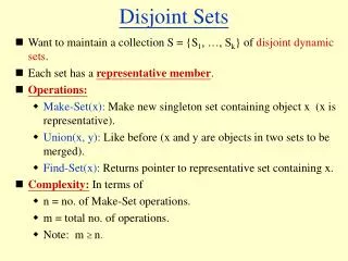
3. Disjoint Sets • Suppose we have N distinct items. We want to partition the items into a collection of sets such that: • each item is in a set • no item is in more than one set • Examples • BU students according to majors, or • BU students according to GPA, or • Graph vertices according to connected components • The resulting sets are said to be disjoint sets.

4. Disjoint sets • Set : a collection of (distinguishable) elements • Two sets are disjoint if they have no common elements • Disjoint-set data structure: • maintains a collection of disjoint sets • each set has a representative element • supported operations: • MakeSet(x) • Find(x) • Union(x,y)

5. Disjoint sets • MakeSet(x) • Given object x, create a new set whose only element (and representative) is pointed to by x • Find(x) • Given object x, return (a pointer to) the representative of the set containing x • Assumption: there is a pointer to each x so we never have to look for an element in the structure

6. Disjoint sets • Union(x,y) • Given two elements x, y, merge the disjoint sets containing them. • The original sets are destroyed. • The new set has a new representative (usually one of the representatives of the original sets) • At most n-1 Unions can be performed where n is the number of elements (why?)

7. Union-Find Algorithms Disjoint set algorithms are sometimes called union-find algorithms.

8. Disjoint Set Example Find the connected components of the undirected graph G=(V,E) (maximal subgraphs that are connected). for (each vertex v in V) Makeset(v): put v in its own set for (each edge (u,v) in E) if (find(u) ~= find(v)) union(u,v) Now we can find if two vertices x and y are in the same connected component by testing find(x) == find(y)

9. Disjoint sets -- implementation In the discussion that follows: • n is the total number of elements (in all sets). • m is the total number of operations performed

10. Disjoint Sets:Implementation #1 • Using linked lists: • The first element of the list is the representative • Each node contains: • an element • a pointer to the next node in the list • a pointer to the representative

11. Disjoint Sets: Implementation#1 • Using linked lists: • MakeSet(x) • Create a list with only one node, for x • Time O(1) • Find(x) • Return the pointer to the representative(assuming you are pointing at the x node) • Time O(1)

12. Disjoint Sets:Implementation#1 • Using linked lists: • Union(x,y) • . Append y’s list to x’s list. • . Pick x as a representative • . Update y’s “representative” pointers • A sequence of m operations may take O(m2) time • Improvement: let each representative keep track of the length of its list and always append the shorter list to the longer one. • Now, a sequence of m operations takes O(m+nlgn) time (why?)

13. Disjoint Sets:Implementation#1An Improvement • Let each representative keep track of the length of its list and always append the shorter list to the longer one. • Theorem: Any sequence of m operations takes O(m+n log n) time.

14. A Tight Bound • O(n + u log u + f), where u and f are, respectively, the number of union and find operations in the sequence of requests • Can we do better?

15. H X F A W B R Up-Trees • A simple data structure for implementing disjoint sets is the up-tree. H, A and W belong to the same set. H is the representative X, B, R and F are in the same set. X is the representative

16. 5 4 13 2 9 11 30 5 13 4 11 13 4 5 2 9 9 11 30 2 30 A Set As A Tree • S = {2, 4, 5, 9, 11, 13, 30} • Some possible tree representations:

17. Operations in Up-Trees Find is easy. Just follow pointer to representative element. The representative has no parent. find(x) • if (parent(x) exists)// not the root return(find(parent(x)); • else return (x); Worst case, height of the tree

18. 13 4 5 9 11 30 2 Steps For find(i) • Start at the node that represents element i and climb up the tree until the root is reached • Return the element in the root • To climb the tree, each node must have a parent pointer

19. 4 2 9 11 30 5 13 Result Of A Find Operation • find(i) is to identify the set that contains element i • In most applications of the union-find problem, the user does not provide set identifiers • The requirement is that find(i) and find(j) return the same value iff elements i and j are in the same set find(i) will return the element that is in the tree root

20. Possible Node Structure • Use nodes that have two fields: element and parent • Use an array table[] such that table[i] is a pointer to the node whose element is i • To do a find(i) operation, start at the node given by table[i] and follow parent fields until a node whose parent field is null is reached • Return element in this root node

21. 13 4 5 9 11 30 2 1 table[] 0 5 10 15 Example (Only some table entries are shown.)

22. 13 4 5 9 11 30 2 1 Better Representation • Use an integer array parent[] such that parent[i] is the element that is the parent of element i parent[] 2 9 13 13 4 5 0 0 5 10 15

23. Union • Union is more complicated. • Make one representative element point to the other, but which way? Does it matter? • In the example, some elements are now deeper away from the root

24. Union(H, X) H X F X points to H B, R and F are now deeper A W B R H X F H points to X A and W are now deeper A W B R

25. Union public union(rootA, rootB) {parent[rootB] = rootA;} • Time Complexity: O(1)

26. A worse case for Union Union can be done in O(1), but may cause find to become O(n) A B C D E Consider the result of the following sequence of operations: Union (A, B) Union (C, A) Union (D, C) Union (E, D)

27. Two Heuristics • There are two heuristics that improve the performance of union-find. • Union by weight or height • Path compression on find

28. 7 13 4 5 8 3 22 6 9 11 30 10 2 1 20 16 14 12 Height Rule • Make tree with smaller height a subtree of the other tree • Break ties arbitrarily union(7,13)

29. 7 13 4 5 8 3 22 6 9 11 30 10 2 1 20 16 14 12 Weight Rule • Make tree with fewer number of elements a subtree of the other tree • Break ties arbitrarily union(7,13)

30. Implementation • Root of each tree must record either its height or the number of elements in the tree. • When a union is done using the height rule, the height increases only when two trees of equal height are united. • When the weight rule is used, the weight of the new tree is the sum of the weights of the trees that are united.

31. Height Of A Tree • If we start with single element trees and perform unions using either the height or the weight rule. The height of a tree with p elements is at most floor (log2p) + 1. • Proof is by induction on p.

32. Union by Weight Heuristic Always attach smaller tree to larger. union(x,y) rep_x = find(x); rep_y = find(y); if (weight[rep_x] < weight[rep_y]) A[rep_x] = rep_y; weight[rep_y] += weight[rep_x]; else A[rep_y] = rep_x; weight[rep_x] += weight[rep_y];

33. Performance w/ Union by Weight • If unions are done by weight, the depth of any element is never greater than log n + 1. • Inductive Proof: • Initially, ever element is at depth zero. • When its depth increases as a result of a union operation (it’s in the smaller tree), it is placed in a tree that becomes at least twice as large as before (union of two equal size trees). • How often can each union be done? -- lg n times, because after at most lg n unions, the tree will contain all n elements. • Therefore, find becomes O(log n) when union by weight is used -- even without path compression.

34. Path Compression Each time we do a find on an element E, we make all elements on path from root to E be immediate children of root by making each element’s parent be the representative. find(x) if (A[x]<0) return(x); A[x] = find(A[x]); return (A[x]); When path compression is done, a sequence of m operations takes O(m log n) time. Amortized time is O(log n) per operation.

35. 7 13 8 3 22 6 4 5 9 g 10 f 11 30 e 2 20 16 14 12 d 1 a, b, c, d, e, f, and g are subtrees a b c Path Compression • find(1) • Do additional work to make future finds easier

36. 7 13 8 3 22 6 4 5 9 g 10 f 11 30 e 2 20 16 14 12 d 1 a, b, c, d, e, f, and g are subtrees a b c Path Compression • Make all nodes on find path point to tree root. • find(1) Makes two passes up the tree

37. Ackermann’s Functions • The Ackermann’s function is the simplest example of a well-defined total function which is computable but not primitive recursive. • "A function to end all functions" -- Gunter Dötzel. • 1. If m = 0 then A(m, n) = n + 1 • 2. If n = 0 then A(m, n) = A(m-1, 1) • 3. Otherwise, A(m, n) = A(m-1, A(m, n-1)) • The function f(n) = A(n, n) grows much faster than polynomials or exponentials or any function that you can imagine

38. Ackermann’s Function • Ackermann’s function. • A(m,n) = 2n, m = 1 and n >= 1 • A(m,n) = A(m-1,2), m>= 2 and n = 1 • A(m,n) = A(m-1,A(m,n-1)), m,n >= 2 • Ackermann’s function grows very rapidly as m and n increase • A(2,4) = 265,536

39. Time Complexity • Inverse of Ackermann’s function. • a(n) = min{k>=1 | A(k,1) > n}, • The inverse function grows very slowly • a(n) < 5 until n = 2A(4,1) + 1 • A(4,1) >> 1080 • For all practical purposes, a (n) < 5

40. Time Complexity Theorem 12.2 [Tarjan and Van Leeuwen] Let T(n,m) be the maximum time required to process any intermixed sequence of n finds and unions. T(n,m) = O(m a (n)) when we start with singleton sets and use either the weight or height rule for unions and any one of the path compression methods for a find.