Download
1 / 51
510 likes | 693 Vues
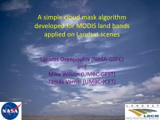
A simple cloud mask algorithm developed for MODIS land bands applied on Landsat scenes Lazaros Oreopoulos (NASA-GSFC) and Mike Wilson (UMBC-GEST) Tamás Várnai (UMBC-JCET). Modified Luo et al. (2008) LTK scheme. I Input Top-of-Atmosphere Reflectance for

E N D
A simple cloud mask algorithm developed for MODIS land bands applied on Landsat scenes Lazaros Oreopoulos (NASA-GSFC) and Mike Wilson (UMBC-GEST) Tamás Várnai (UMBC-JCET)
Modified Luo et al. (2008) LTK scheme IInput Top-of-Atmosphere Reflectance for LandSat Bands 1, 3, 4, and 5. (L1, L3, L4, and L5) Yes Non-Vegetated Lands L1<L3 and L3<L4 and L4<L5*1.07 and L5<0.65 or L1*0.8<L3 and L3<L4*0.8 and L4<L5 and L3<0.22 No Yes Snow/Ice L3>0.24 and L5<0.16 and L3>L4 or 0.24>L3>0.18 and L5<L3-0.08 and L3>L4 No Yes Water Bodies L3>L4 and L3>L5*0.67 and L1<0.30 and L3<0.20 or L3>L4*0.8 and L3>L5*0.67 and L3<0.06 No Yes Clouds [L1>0.15(0.20) or L3>0.18] and L5>0.12 (0.16) and max(L1,L3)>L5*0.67 No Vegetated Lands No thermal!
Subtropical South P158_r72_4 Non-Vegetated Lands Snow/Ice ACCA agreement 95.4% LTK agreement 91.5% Water Bodies Vegetated Lands Cloud
Performance comparison between LTK and ACCA Irish et al. scenes via USGS and BU
Some facts about our “poor” (19/156) scenes “poor” = either errors in scene CF > 10% or level of mask agreement < 80% • 5 are from south pole latitude zone • 7 have >10 % error in manual scene CF between Irish et al. and USGS • 7 (3 from above) have also ACCA scene CF errors > 10%, i.e, 11 “bad” scenes • From 11, 6 have < 80% mask agreement for ACCA, and 7 do not belong to BU dataset • 12/19 have thin cloud amount above the median (0.31) of 134/156 scenes with some cloud
Subtropical North, Path 31, Row 43 RGB (5-4-3)
Subtropical North, Path 31, Row 43 LEGEND Land Cloud Projection, of 12 km cloud no shadow Resembles shadow, no nearby cloud Cloud shadow detected If over vegetated/non-vegetated land: Max(R4,R5)/R1<1.5 R3<0.12 R4<0.24 R5<0.24 If over snow: R4/R1<0.75
MODIS 2006240 19:45 UTC (courtesy of R. Frey) Band 26 (1.38µm) Band 31 (11.1µm)
MODIS 2006240 19:45 UTC (courtesy of R. Frey) 1.38 µm Ref. Test (black means test not performed) Split-window Test
Thresholding the Split Window • The difference in Brightness Temperature between 11 µm and 12 µm is calculated for gridded ECMWF data. • ECMWF is on 2.5 degree longitude by 2.5 degree latitude grid. • All data taken at 00 Z on January 15, 2002. • Total of 10512 different profiles, each with information on pressure, height, temperature, ozone, and water vapor. • Converted to an equal area grid, so that polar regions are not unfairly emphasized; 6454 profiles remained for analysis.
Selected profiles shown by triangles Fewer Triangles occur near the poles
Simulations with clouds at tropopause • A cloud of a given optical depth (0.1, 0.3, 0.5, 0.75, 1, 2, 3, 4) was placed in each of 6454 profiles at the calculated tropopause level (where the lapse rate dropped below 2 K/km) • 8 tropopause layers were possible: • 500 mb – 400 mb • 400 mb – 300 mb • 300 mb – 250 mb • 250 mb – 200 mb • 200 mb – 150 mb • 150 mb – 100 mb • 100 mb – 70 mb • 70 mb – 50 mb
Simulations From the CASPR User’s guide