
From last lecture
E N D
Presentation Transcript
From last lecture • We want to find a fixed point of F, that is to say a map m such that m = F(m) • Define ?, which is ? lifted to be a map: ? = e. ? • Compute F(?), then F(F(?)), then F(F(F(?))), ... until the result doesn’t change anymore
From last lecture • If F is monotonic and height of lattice is finite: iterative algorithm terminates • If F is monotonic, the fixed point we find is the least fixed point.
What about if we start at top? • What if we start with >: F(>), F(F(>)), F(F(F(>))) • We get the greatest fixed point • Why do we prefer the least fixed point? • More precise
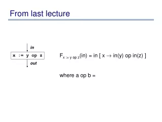
Graphically y 10 10 x
Graphically y 10 10 x
Graphically y 10 10 x
Another example: constant prop • Set D = in x := N Fx := n(in) = out in x := y op z Fx := y op z(in) = out
Another example: constant prop • Set D = 2 { x ! N | x 2 Vars Æ N 2 Z } in x := N Fx := n(in) = in – { x ! * } [ { x ! N } out in x := y op z Fx := y op z(in) = in – { x ! * } [ { x ! N | ( y ! N1 ) 2 in Æ ( z ! N2 ) 2 in Æ N = N1 op N2 } out
Another example: constant prop in Fx := *y(in) = x := *y out in F*x := y(in) = *x := y out
Another example: constant prop in Fx := *y(in) = in – { x ! * } [ { x ! N | 8 z 2 may-point-to(x) . (z ! N) 2 in } x := *y out in F*x := y(in) = in – { z ! * | z 2 may-point(x) } [ { z ! N | z 2 must-point-to(x) Æ y ! N 2 in } [ { z ! N | (y ! N) 2 in Æ (z ! N) 2 in } *x := y out
Another example: constant prop in *x := *y + *z F*x := *y + *z(in) = out in x := f(...) Fx := f(...)(in) = out
Another example: constant prop in *x := *y + *z F*x := *y + *z(in) = Fa := *y;b := *z;c := a + b; *x := c(in) out in x := f(...) Fx := f(...)(in) = ; out
Another example: constant prop in s: if (...) out[0] out[1] in[0] in[1] merge out
Lattice • (D, v, ?, >, t, u) =
Lattice • (D, v, ?, >, t, u) = (2 { x ! N | x 2 Vars Æ N 2 Z } , w, D, ;, u, t)
Example x := 5 v := 2 w := 3 y := x * 2 z := y + 5 x := x + 1 w := v + 1 w := w * v
Better lattice • Suppose we only had one variable
Better lattice • Suppose we only had one variable • D = {?, > } [ Z • 8 i 2 Z . ?v i Æ i v> • height = 3
For all variables • Two possibilities • Option 1: Tuple of lattices • Given lattices (D1, v1, ?1, >1, t1, u1) ... (Dn, vn, ?n, >n, tn, un) create: tuple lattice Dn =
For all variables • Two possibilities • Option 1: Tuple of lattices • Given lattices (D1, v1, ?1, >1, t1, u1) ... (Dn, vn, ?n, >n, tn, un) create: tuple lattice Dn = ((D1£ ... £ Dn), v, ?, >, t, u) where ? = (?1, ..., ?n) > = (>1, ..., >n) (a1, ..., an) t (b1, ..., bn) = (a1t1 b1, ..., antn bn) (a1, ..., an) u (b1, ..., bn) = (a1u1 b1, ..., anun bn) height = height(D1) + ... + height(Dn)
For all variables • Option 2: Map from variables to single lattice • Given lattice (D, v, ?, >, t, u) and a set V, create: map lattice V ! D = (V ! D, v, ?, >, t, u)
Back to example in Fx := y op z(in) = x := y op z out
Back to example in Fx := y op z(in) = in [ x ! in(y) op in(z) ] where a op b = x := y op z out
General approach to domain design • Simple lattices: • boolean logic lattice • powerset lattice • incomparable set: set of incomparable values, plus top and bottom (eg const prop lattice) • two point lattice: just top and bottom • Use combinators to create more complicated lattices • tuple lattice constructor • map lattice constructor
May vs Must • Has to do with definition of computed info • Set of x ! y must-point-to pairs • if we compute x ! y, then, then during program execution, x must point to y • Set of x! y may-point-to pairs • if during program execution, it is possible for x to point to y, then we must compute x ! y
Direction of analysis • Although constraints are not directional, flow functions are • All flow functions we have seen so far are in the forward direction • In some cases, the constraints are of the form in = F(out) • These are called backward problems. • Example: live variables • compute the of variables that may be live
Example: live variables • Set D = • Lattice: (D, v, ?, >, t, u) =
Example: live variables • Set D = 2 Vars • Lattice: (D, v, ?, >, t, u) = (2Vars, µ, ; ,Vars, [, Å) in Fx := y op z(out) = x := y op z out
Example: live variables • Set D = 2 Vars • Lattice: (D, v, ?, >, t, u) = (2Vars, µ, ; ,Vars, [, Å) in Fx := y op z(out) = out – { x } [ { y, z} x := y op z out
Example: live variables x := 5 y := x + 2 y := x + 10 x := x + 1 ... y ...
Example: live variables x := 5 y := x + 2 y := x + 10 x := x + 1 ... y ...
Theory of backward analyses • Can formalize backward analyses in two ways • Option 1: reverse flow graph, and then run forward problem • Option 2: re-develop the theory, but in the backward direction
Precision • Going back to constant prop, in what cases would we lose precision?
Precision • Going back to constant prop, in what cases would we lose precision? if (...) { x := -1; } else x := 1; } y := x * x; ... y ... if (p) { x := 5; } else x := 4; } ... if (p) { y := x + 1 } else { y := x + 2 } ... y ... x := 5 if (<expr>) { x := 6 } ... x ... where <expr> is equiv to false
Precision • The first problem: Unreachable code • solution: run unreachable code removal before • the unreachable code removal analysis will do its best, but may not remove all unreachable code • The other two problems are path-sensitivity issues • Branch correlations: some paths are infeasible • Path merging: can lead to loss of precision
MOP: meet over all paths • Information computed at a given point is the meet of the information computed by each path to the program point if (...) { x := -1; } else x := 1; } y := x * x; ... y ...
MOP • For a path p, which is a sequence of statements [s1, ..., sn] , define: Fp(in) = Fsn( ...Fs1(in) ... ) • In other words: Fp = • Given an edge e, let paths-to(e) be the (possibly infinite) set of paths that lead to e • Given an edge e, MOP(e) = • For us, should be called JOP...
MOP vs. dataflow • As we saw in our example, in general,MOP dataflow • In what cases is MOP the same as dataflow? x := -1; y := x * x; ... y ... x := 1; y := x * x; ... y ...
MOP vs. dataflow • As we saw in our example, in general,MOP dataflow • In what cases is MOP the same as dataflow? • Distributive problems. A problem is distributive if: 8 a, b . F(a t b) = F(a) t F(b)
Summary of precision • Dataflow is the basic algorithm • To basic dataflow, we can add path-separation • Get MOP, which is same as dataflow for distributive problems • Variety of research efforts to get closer to MOP for non-distributive problems • To basic dataflow, we can add path-pruning • Get branch correlation • Will see example of this later in the course • To basic dataflow, can add both: • meet over all feasible paths