Download

1 / 28
280 likes | 483 Vues
Professor XXX Course Name / #. Efficient Risky Portfolios. Variance of return - a poor measure of risk. Investors can only expect compensation for systematic risk Asset pricing models aim to define and quantify systematic risk.

E N D
Professor XXX Course Name / #
Efficient Risky Portfolios Variance of return - a poor measure of risk • Investors can only expect compensationfor systematic risk • Asset pricing models aim to define andquantify systematic risk Begin developing pricing model by asking:Are some portfolios better than others?
Expanding The Feasible Set On The Efficient Frontier EF including domestic & foreign assets E(RP) EF including domestic stocks, bonds, and real estate EF for portfolios of domestic stocks P
N – Asset Portfolios efficient portfolios • • Stock B F efficient portfolios • • • E • • • • • • • C (50%A, 50%B) • • • D • • • • MVP (75%A, 25%B) MVP • Stock A inefficient portfolios Are Some Portfolios Better Than Others? Efficient portfolios achieve the highest possible return for any level of volatility Two – Asset Portfolios E(RP) P What happens when we add a risk-free asset to the picture?
Expected Return (per month) and Standard Deviation for Various Portfolios
Expected return = 10% Risky asset X Three possible returns:-10%; 10%; 30% Standard deviation =16.3% Risk-free asset Y Return: 6% Buying asset Y = Lending money at 6% interest Expected return = 8% $100 Asset X $100 Asset Y Three possible returns:-2%; 8%; 18% Standard deviation =8.16% Riskless Borrowing And Lending • How would a portfolio with $100 (50%) in asset X and $100 (50%) in asset Y perform? Portfolio has lower return but also less volatility than 100% in X Portfolio has higher return and higher volatility than 100% in risk-free
When X Pays –10% When X Pays 10% When X Pays 30% Riskless Borrowing And Lending (Continued) • What if we sell short asset Y instead of buying it?Borrow $100 at 6%Must repay $106 Invest $300 in X Original $200 investment plus $100 in borrowed funds Expected return on the portfolio is 12%. Higher expected return comes at the expense of greater volatility
The more we invest in X, the higher the expected return The expected return is higher, but so is the volatility This relationship is linear Riskless Borrowing And Lending (Continued)
Portfolios Of Risky & Risk-Free Assets E(RP) borrowing • 16.5% B • 12% lending MF • 9% A • RF=6% P 15% 0 30% 52%
Suppose investors agree on which portfolio is efficient Equilibrium requires this to be the Market Portfolio Market Portfolio: value weighted portfolio of all available risky assets The Market Portfolio Only one risky portfolio is efficient The line connecting Rf to the market portfolio - called the Capital Market Line
Finding the Optimal Risky Portfolio • If investors can borrow and lend at the risk-free rate, then from the entire feasible set of risky portfolios, one portfolio will emerge that maximizes the return investors can expect for a given standard deviation. • To determine the composition of the optimal portfolio, you need to know the expected return and standard deviation for every risky asset, as well as the covariance between every pair of assets.
The Capital Market Line • The line connecting Rf to the market portfolio is called the Capital Market Line (CML) • CML quantifies the relationship between the expected return and standard deviation for portfolios consisting of the risk-free asset and the market portfolio, using
Capital Asset Pricing Model (CAPM) Only beta changes from one security to the next. For that reason, analysts classify the CAPM as a single-factor model, meaning that just one variable explains differences in returns across securities.
The Security Market Line • Plots the relationship between expected return and betas • In equilibrium, all assets lie on this line • If stock lies above the line • Expected return is too high • Investors bid up price until expected return falls • If stock lies below the line • Expected return is too low • Investors sell stock, driving down price until expected return rises
A - Undervalued • • A B • • B - Overvalued The Security Market Line E(RP) SML Slope = E(Rm) - RF = MarketRisk Premium (MRP) RM • • RF • =1.0 i
Beta • The numerator is the covariance of the stock with the market • The denominator is the market’s variance In the CAPM, a stock’s systematic risk is captured by beta The higher the beta, the higher the expected return on the stock
E(Ri) = Rf + ß [E(Rm) – Rf] • Return for bearing no market risk • Stock’s exposure to market risk • Reward for bearing market risk Beta And Expected Return Beta measures a stock’s exposure to market risk The market risk premium is the reward for bearing market risk: • Rm - Rf
Calculating Expected Returns E(Ri) = Rf + ß [E(Rm) – Rf] • Assume • Risk–free rate = 2% • Expected return on the market = 8% When Beta = 0, The Return Equals The Risk-Free Return When Beta = 1, The Return Equals The Expected Market Return
Using The Security Market Line The SML and where P&G and GE place on it r% SML 15 12.4% slope = E(Rm) – RF = MRP = 10% - 2% = 8% = Y ÷ X • 10 6.8% 5 Rf = 2% P&G 1 GE 2
Shifts In The SML Due To A Shift In Required Market Return r% SML1 15 SML2 11.1% • Shift due to change in market risk premium from 8% to 7% 10 • 6.2% 5 Rf = 2% P&G 1 GE 2
Shifts In The SML Due To A Shift In The Risk-Free Rate SML2 r% SML1 15 14.4% Shift due to change in risk-free rate from 2% to 4%, with market risk premium remaining at 8%. Note all returns increase by 2% • 10 8.8% 5 Rf = 4% P&G 1 GE 2
Alternatives To CAPM • Arbitrage Pricing Theory • Fama-French Model Betas represent sensitivities to each source of risk Terms in parentheses are the rewards for bearing each type of risk.
The Current State of APT • Investors demand compensation for taking risk because they are risk averse. • There is widespread agreement that systematic risk drives returns. • You can measure systematic risk in several different ways depending on the asset pricing model you choose. • The CAPM is still widely used in practice in both corporate finance and investment-oriented professions.