Making Inferences about Causality

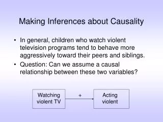
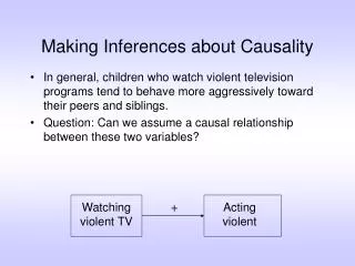
1. Watching violent TV Acting violent Making Inferences about Causality • In general, children who watch violent television programs tend to behave more aggressively toward their peers and siblings. • Question: Can we assume a causal relationship between these two variables? +

2. Making Inferences about Causality • Answer: not necessarily • Although causality generally implies correlation, correlation does not necessarily imply causality. • There are at least three other ways to explain the correlation between TV viewing and aggressive behavior.

3. Watching violent TV Acting violent Making Inferences about Causality (a) Acting aggressively makes you want to watch more violent TV. +

4. Watching violent TV Acting violent Making Inferences about Causality (b) Acting violent makes you want to watch more TV and watching TV makes you act more violently. + +

5. Watching violent TV Living in a violent family Acting violent Making Inferences about Causality (c) A “third variable” influences both variables, causing them to be correlated. + +

6. How can we tease apart these various possibilities? • One way to do so is to conduct an experiment. • In an experiment, at least one variable is manipulated (i.e., systematically varied) by the researcher in order to study its effects on another variable.

7. Watching violent TV Acting violent Experimental Research • Features of an experiment (a) At least one variable is manipulated or varied by the experimenter: independent variable (IV) (b) The variable presumably affected by the manipulation is called the dependent variable (DV) (c) random assignment to conditions IV DV +

8. Dependent Variable: Aggressive behavior Number of times the child punches his or her peers on the playground IV DV • Independent Variable: Watching violent TV • Levels: • view an episode of the Sopranos • view an episode of the Sopranos in which the violent scenes have been edited

9. Random Assignment • Why is random assignment important? • Consider what would happen if we assigned men to the “violent” level of the IV and women to the “non-violent” level of the IV. • Sex would be correlated with the IV.

10. Random Assignment • Confounding variable: a variable that influences the dependent variable and is associated with the independent variable • When confounding variables are present, we cannot make a strong inference that the independent variable causes the dependent variable.

11. Random Assignment • Random assignment to conditions helps to remove the problem of confounding variables. • When people are randomly assigned to conditions, we should (in the long run) have equal numbers of men and women in our two conditions. • As a result of random assignment, the possible confound (e.g., sex) is uncorrelated with the independent variable.

12. Random Assignment • Previously, we had discussed the possibility that the violence of the family context is a “third variable” that might be causing both violent TV viewing and aggressive behavior. • We could control for this possible confound by randomly assigning people to violent TV viewing conditions. • Theoretically, there should be an equal number of people from violent families in each condition.

13. Confounding Variables and Non-Confounding Variables • A variable can exist that has a genuine effect on the dependent variable but that is uncorrelated with the independent variable. • Such cases create noise, but are not confounds per se.

14. Watching violent TV Acting violent Confounding Variables and Non-confounding Variables Acting violent + + + + Living in a violent family Living in a violent family Watching violent TV

15. Causal inferences • Up to this point we have been discussing ways to make inferences about the causal relationships between variables. • One of the strongest ways to make causal inferences is to conduct an experiment (i.e., systematically manipulate a variable to study its effect on another).

16. Causal inferences • Unfortunately, we cannot experimentally study a lot of the important questions in personality psychology for practical or ethical reasons. • For example, if we’re interested in how people’s prior experiences in close relationships might influence their future relationships, we can’t use an experimental design to manipulate the kinds of relational experiences that people have.

17. Causal inferences • How can we make inferences about causality in these circumstances? • There is no fool-proof way of doing so, but today we’ll discuss some techniques that are commonly used. • control by selection • statistical control

18. Control by selection • The biggest problem with inferring causality from correlations is the third variable problem. For any relationship we may study in psychology, there are a number of confounding variables that may interfere with our ability to make the correct causal inference.

19. Control by selection • Stanovich, a psychologist, has described an interesting example involving public versus private schools. • It has been established empirically that children attending private schools perform better on standardized tests than children attending public schools. • Many people believe that sending children to private schools will help increase test scores. + “quality” of school test scores

20. Control by selection • One of the problems with this inference is that there are other variables that could influence both the kind of school a kid attends and his or her test scores. • For example, the financial status of the family is a possible confound. “quality” of school test scores + + financial status

21. Control by selection • Recall that a confounding variable is one that is associated with both the dependent variable (i.e., test scores) and the independent variable (i.e., type of school). • Thus, if we can create a situation in which there is no variation in the confounding variable, we can remove its potential effects on the other variables of interest.

22. Control by selection • To do this, we might select a sample of students who come from families with the same financial status. • If there is a relationship between “quality” of school and test scores in this sample, then we can be reasonably certain that it is not due to differences in financial status because everyone in the sample has the same financial status.

23. Control by selection • In short, when we control confounds via sample selection, we are identifying possible confounds in advance and controlling them by removing the variability in the possible confound. • One limitation of this approach is that it requires that we know in advance all the confounding variables. In an experimental design with random assignment, we don’t have to worry too much about knowing exactly what the confounds could be.

24. Statistical control • Another commonly used method for controlling possible confounds involves statistical techniques, such as multiple regressionandpartial correlation. • In short, this approach is similar to what we just discussed. However, instead of selecting our sample so that there is no variation in the confounding variable, we use statistical techniques that essentially remove the effects of the confounding variable.

25. Statistical control • If you know the correlations among three variables (e.g, X, Y, and Z), you can compute a partial correlation, rYZ.X. A partial correlation characterizes the correlation between two variables (e.g., Y and Z) after statistically removing their association with a third variable (e.g., X).

26. Statistical control • If this diagram represents the “true” state of affairs, then here are correlations we would expect between these three variables: Y Z “quality” of school test scores .5 .5 financial status • We expect Y and Z to correlate about .25 even though one doesn’t cause the other. X

27. Statistical control Y Z “quality” of school test scores .5 .5 financial status • The partial correlation between Y and Z is 0, suggesting that there is no relationship between these two variables once we control for the confound. X

28. Statistical control • What happens if we assume that quality of school does influence student test scores? • Here is the implied correlation matrix for this model: Y Z .5 “quality” of school test scores .5 .5 financial status X

29. Statistical control Y Z .5 “quality” of school test scores .5 .5 financial status • The partial correlation is .65, suggesting that there is still an association between Y and Z after controlling X. X

30. Statistical control • Like “control by selection,” statistical control is not a foolproof method. If there are confounds that have not been measured, these can still lead to a correlation between two variables. • In short, if one is interested in making causal inferences about the relationship between two variables in a non-experimental context, it is wise to try to statistically control possible confounding variables.