Download
1 / 27
270 likes | 683 Vues
A Morphable Model For The Synthesis Of 3D Faces. Volker Blanz Thomas Vetter. OUTLINE. Introduction Related work Database Morphable 3D Face Model Matching a morphable model to images/3D scans Building a morphable model Results Future work. Introduction.

E N D
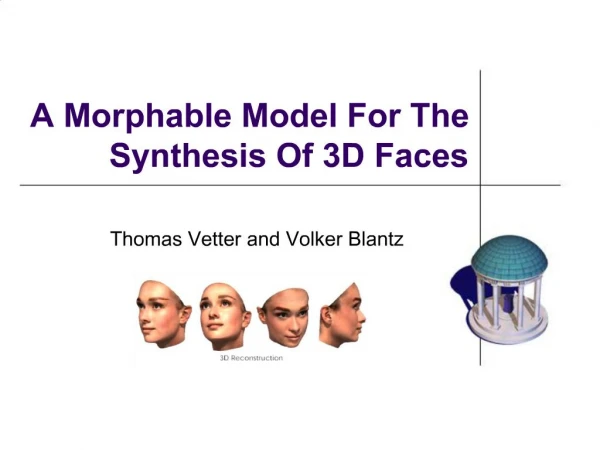
A Morphable Model For The Synthesis Of 3D Faces Volker Blanz Thomas Vetter
OUTLINE • Introduction • Related work • Database • Morphable 3D Face Model • Matching a morphable model to images/3D scans • Building a morphable model • Results • Future work
Introduction • Computer aided modeling of human faces still requires a great deal of expertise and manual control to avoid unrealistic, non-face-like results. • Most limitations of automated techniques for face synthesis face animation or for general changes in the appearance of an individual face can be described as the problem of finding corresponding feature locations in different faces.
Introduction • In this paper, we present a parametric face modeling technique that assists in both problems. • First, arbitrary human faces can be created simultaneously controlling the likelihood of the generated faces. • Second, the system is able to compute correspondence between new faces. • We developed an algorithm that adjusts the model parameters automatically for an optimal reconstruction of the target, requiring only a minimum of manual initialization.
Related work • The correspondence problem between different three-dimensional face data has been addressed previously by Lee et al.[20]. • First, we compute the correspondence in high resolution, considering shape and texture data simultaneously. • Second, instead of using a physical tissue model to constrain the range of allowed mesh deformations, we use the statistics of our example faces to keep deformations plausible. • Third, we do not rely on routines that are specifically designed to detect the features exclusively found in faces, e.g., eyes, nose.
Related work • Finding the correspondence • Optical flow • [35] T. Vetter and V. Blanz. “Estimating coloured 3d face models from single images: An example based approach.” • Bootstrapping • [36] T. Vetter, M. J. Jones, and T. Poggio. “A bootstrapping algorithm for learning linear models of object classes.”
Database • Laser scans of 200 heads of young adults (100 male and 100 female) were used. • The laser scans provide head structure data in a cylindrical representation, with radii r(h, φ) of surface points sampled at 512 equally-spaced angles φ, and at 512 equally spaced vertical steps h. • The RGB-color values R(h, φ),G(h, φ),B(h, φ), were recorded in the same spatial resolution and were stored in a texture map with 8 bit per channel. • The resultant faces were represented by approximately 70,000 vertices and the same number of color values.
Morphable 3D face model • We represent the geometry of a face with a shape-vector S=(X1,Y1,Z1,X2,Y2,…,Xn,Yn,Zn)T ,that contains the X,Y,Z-coordinates of its n vertices. • We represent the texture of a face by a texture-vector T =(R1,G1,B1,R2,G2,…,Rn,Gn,Bn)T , that contains the R,G,B color values of the n corresponding vertices. • Since we assume all faces in full correspondence, new shapes Smodel and new textures Tmodel can be expressed as a linear combination of the shapes and textures of the m exemplar faces.
Morphable 3D face model • We fit a multivariate normal distribution to our data set of 200 faces, based on the averages of shape and texture and the covariance matrices Cs and Ct. • A common technique for data compression known as Principal Component Analysis (PCA) performs a basis transformation to an orthogonal coordinate system formed by the eigenvectors si and ti of the covariance matrices.
Morphable 3D face model • Segmented morphable model: The morphable model describedin equation (1), has m-1 degrees of freedom for texture and shape. • The expressiveness of the model can be increased by dividing faces into independent sub-regions that are morphed independently, for example into eyes, nose, mouth and a surrounding region. • A complete 3D face is generated by blending them at the borders
Morphable 3D face model • Facial attributes • Some facial attributes can easily be related to biophysical measurements, such as the width of the mouth, facial femininity or being more or less bony can hardly be described by numbers. • Unlike facial expressions, attributes that are invariant for each individual are more difficult to isolate. The following method allows us to model facial attributes such as gender, fullness of faces, darkness of eyebrows, double chins, and hooked versus concave noses
Morphable 3D face model • Based on a set of faces (Si,Ti) with manually assigned labels μi describing the markedness of the attribute, we compute weighted sums • Multiples of (ΔS, ΔT) can now be added to or subtracted from any individual face.
Matching a morphable model to images • Coefficients of the 3D model are optimized along with a set of rendering parameters such that they produce an image as close as possible to the input image. • It starts with the average head and with rendering parameters roughly estimated by the user.
Matching a morphable model to images • Model Parameters: Facial shape and texture are defined by coefficients αj and βj ,j = 1,2,…,m-1. • Rendering parameters contain camera position (azimuth and elevation), object scale, image plane rotation and translation, intensity ir,amb,ig,amb,ib,amb of ambient light, and intensity ir,dir,ig,dir,ib,dir of directed light
Matching a morphable model to images • From parameters , colored images are rendered using perspective projection and the Phong illumination model. • The reconstructed image is supposed to be closest to the input image in terms of Euclidean distance
Matching a morphable model to images • In terms of Bayes decision theory, the problem is to find the set of parameters with maximum posterior probability, given an image Iinput. Whileand rendering parameters completely determine the predicted image Imodel , the observed image Iinput may vary due to noise. • For Gaussian noise with a standard deviation , the likelihood to observe Iinput is • Maximum posterior probability is then achieved by minimizing the cost function
Matching a morphable model to images • The optimization algorithm described below uses an estimate of E based on a random selection of surface points. In the center of triangle k, texture (Rk,Gk,Bk)T and 3D location (Xk,Yk,Zk)T are averages of the values at the corners. Perspective projection maps these points to image locations (px,k,py,k)T . • According to Phong illumination, the color componentsIr,model,Ig,model and Ib,model take the form
Matching a morphable model to images • For high resolution 3D meshes, variations in Imodel across each triangle are small, so EI may be approximated by where ak is the image area covered by triangle k. • In gradient descent, contributions from different triangles of the mesh would be redundant. In each iteration, we therefore select a random subsetof 40 triangles k and replace EI by
Matching a morphable model to images • Parameters are updated depending on analytical derivatives of the cost function E, using and similarly for and , with suitable factors . • Coarse-to-Fine: In order to avoid local minima, the algorithm follows a coarse-to-fine strategy in several respects:a) The first set of iterations is performed on a down-sampled version of the input image with a low resolution morphable model.
Matching a morphable model to images • b) We start by optimizing only the first coefficientsand controlling the first principal components, along with all parameters . In subsequent iterations, more and more principal components are added. • c) Starting with a relatively large , which puts a strong weight on prior probability, is later reduced to obtain maximum matching quality. • d) In the last iterations, the face model is broken down into segments. • Multiple Images • Illumination-Corrected Texture Extraction
Matching a morphable model to 3D scans • Analogous to images, where perspective projection , the laser scans provide a two-dimensional cylindrical parameterization of the surface by means of a mapping => . • Hence, the matching algorithm from the previous section now determines and minimizing
Building a morphable model • In this section, we describe how to build the morphable model from a set of unregistered 3D prototypes, and to add a new face to the existing morphable model, increasing its dimensionality. • Section 4.1 finds the best match of a given face only within the range of the morphable model, it cannot add new dimensions to the vector space of faces. • We use an optic flow algorithm that computes correspondence between two faces without the need of a morphable model.
Building a morphable model • 3D Correspondence using Optic Flow • Initially designed to find corresponding points in grey-level images, a gradient-based optic flow algorithm is modified to establish correspondence between a pair of 3D scans , taking into account color and radius values simultaneously. • The algorithm computes a flow field that minimizes differences ofthat weights variations in texture and shape equally.
Results • We tested the expressive power of our morphable model by automatically reconstructing 3D faces from photographs of arbitrary Caucasian faces of middle age that were not in the database. • The whole matching procedure was performed in 105 iterations. On an SGI R10000 processor,computation time was 50 minutes.
Results • If previously unseen backgrounds become visible, we fill the holes with neighboring background pixels (Fig. 6). • The face can be combined with other 3D graphic objects, such as glasses or hats, and then be rendered in front of the background, computing cast shadows or new illumination conditions (Fig. 7).
Future work • Issues of implementation: We plan to speed up our matching algorithm by implementing a simplified Newton-method for minimizing the cost function (Equation 5). • Extending the database: While the current database is sufficient to model Caucasian faces of middle age, we would like to extend it to children, to elderly people as well as to other races. • Extending the face model: Our current morphable model is restricted to the face area, because a sufficient 3D model of hair cannot be obtained with our laser scanner.