
PRAM Model for Parallel Computation
E N D
Presentation Transcript
PRAM Model for Parallel Computation Chapter 1A: Part 2 of Chapter 1
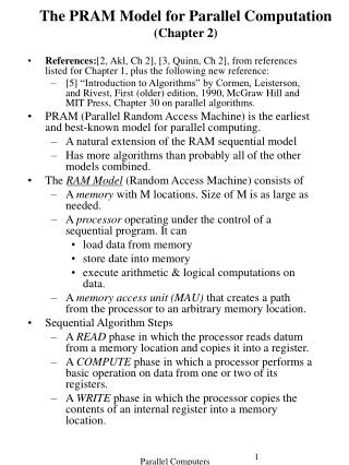
The RAM Model of Computation Revisited • The Random Access Model (or RAM) model for sequential computation was discussed earlier. • Assume that the memory has M memory locations, where M is a large (finite) number • Accessing memory can be done in unit time. • Instructions are executed one after another, with no concurrent operations. • The input size depends on the problem being studied and is the number of items in the input • The running time of an algorithm is the number of primitive operations or steps performed.
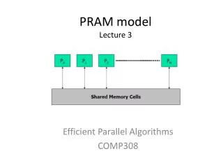
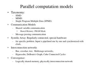
PRAM (Parallel Random Access Machine) • PRAM is a natural generalization of the RAM sequential model. • Each of the p processors P0, P1, … , Pp-1 are identical to a RAM processor and are often referred to as processing elements (PEs) or simply as processors. • All processors can read or write to a shared global memory in parallel (i.e., at the same time). • The processors can also perform various arithmetic and logical operations in parallel • Running time can be measured in terms of the number of parallel memory accesses an algorithm performs.
PRAM Properties • An unbounded number of processors all can access • All processors can access an unbounded shared memory • All processor’s execution steps are synchronized • However, processors can run different programs. • Each processor has an unique id, called the pid • Processors can be instructed to do different things, based on their pid (if pid < 200, do this, else do that)
The PRAM Model • Parallel Random Access Machine • Theoretical model for parallel machines • p processors with uniform access to a large memory bank • UMA (uniform memory access) – Equal memory access time for any processor to any address
The PRAM Models • PRAM models vary according • How they handle write conflicts • The models differ in how fast they can solve various problems. • Exclusive Read, Exclusive Write (EREW) • Only one processor is allow to read or write to the same memory cell during any one step • Concurrent Read Exclusive Write (CREW) • Concurrent Read Concurrent Write (CRCW) • An algorithm that works correctly for EREW will also work correctly for CREW and CRCW, but not vice versa
Summary of Memory Protocols • Exclusive-Read Exclusive-Write • Exclusive-Read Concurrent-Write • Concurrent-Read Exclusive-Write • Concurrent-Read Concurrent-Write • If concurrent write is allowed we must decide which “written value” to accept
Assumptions • There is no upper bound on the number of processors in the PRAM model. • Any memory location is uniformly accessible from any processor. • There is no limit on the amount of shared memory in the system. • Resource contention is absent. • The algorithms designed for the PRAM model can be implemented on real parallel machines, but will incur communication cost. • Since communication and resource costs varies on real machines, PRAM algorithms can be used to establish a lower bound on running time for problems.
P1 Shared Memory P2 P3 . . . PN More Details on the PRAM Model • Both the memory size and the number of processors are unbounded • No direct communication between processors • they communicate via the memory • Every processor accesses any memory location in 1 cycle • Typically all processors execute the same algorithm in a synchronous fashion although each processor can run a different program. • READ phase • COMPUTE phase • WRITE phase • Some subset of the processors can stay idle (e.g., even numbered processors may not work, while odd processors do, and conversely)
PRAM CW? • What ends up being stored when multiple writes occur? • priority CW: processors are assigned priorities and the top priority processor is the one that does writing for each group write • Fail common CW: if values are not equal, no write occurs • Collision common CW: if values not equal, write a “failure value” • Fail-safe common CW: if values not equal, then algorithm aborts • Random CW: non-deterministic choice of which value is written • Combining CW: write the sum, average, max, min, etc. of the values • etc. • For CRCW PRAM, one of the above type CWs is assumed. The CWs can be ordered so that later type CWs can execute the earlier types of CWs. • As shown in the textbook, Parallel Computation: Models & Algorithms” by Selim Akl, a PRAM machine that can perform all of PRAM operations including all CWs can be built with circuits and runs in O(log n) time. • In fact, most PRAM algorithms end up not needing CW.
PRAM Example 1 • Problem: • We have a linked list of length n • For each element i, compute its distance to the end of the list: d[i] = 0 if next[i] = NIL d[i] = d[next[i]] + 1 otherwise • Sequential algorithm is O(n) • We can define a PRAM algorithm running in O(log n) time • Associate one processor to each element of the list • At each iteration split the list in two with odd-placed and even-placed elements in different lists • List size is divided by 2 at each step, hence O(log n)
PRAM Example 1 Principle: Look at the next element Add its d[i] value to yours Point to the next element’s next element 1 1 1 1 1 0 The active processors in each list is reduced by 2 at each step, hence the O(log n) complexity 2 2 2 2 1 0 4 4 3 2 1 0 5 4 3 2 1 0
PRAM Example 1 • Algorithm forall i if next[i] == NIL then d[i] 0 else d[i] 1 while there is an i such that next[i] ≠ NIL forall i if next[i] ≠ NIL then d[i] d[i] + d[next[i]] next[i] next[next[i]] What about the correctness of this algorithm?
forall Loop • At each step, the updates must be synchronized so that pointers point to the right things: next[i] next[next[i]] • Ensured by the semantic of forall • Nobody really writes it out, but one mustn’t forget that it’s really what happens underneath forall i tmp[i] = B[i] forall i A[i] = tmp[i] forall i A[i] = B[i]
while Condition • while there is an i such that next[i] ≠NULL • How can one do such a global test on a PRAM? • Cannot be done in constant time unless the PRAM is CRCW • At the end of above step, each processor could write to a same memory location TRUE or FALSE depending on next[i] being equal to NULL or not, and one can then take the AND of all values (to resolve concurrent writes) • On a PRAM CREW, one needs O(log n) steps for doing a global test like the above • In this case, one can just rewrite the while loop into a for loop, because we have analyzed the way in which the iterations go: for step = 1 to log n
What Type of PRAM? • The previous algorithm does not require a CW machine, but: tmp[i] d[i] + d[next[i] could require a concurrent reads by proc j and k if k=next[j] and k performed the “d[i]” part of execution while j performed the “d[next[i]]” part of this execution • Solution 1: Won’t occur if inline execution is strictly synchronous as d[k] and d[next[j]] will execute at different times • Solution 2: Execute two inline instructions on lines: tmp2[i] d[i] tmp[i] tmp2[i] + d[next[i]] (note that the above are technically in two different steps in each pass through this loop) • Now we have an execution that works on a EREW PRAM, which is the most restrictive type
Final Algorithm on a EREW PRAM forall i if next[i] == NILL then d[i] 0 else d[i] 1 for step = 1 to log n forall i if next[i] ≠ NIL then tmp[i] d[i] d[i] tmp[i] + d[next[i]] next[i] next[next[i]] O(1) O(log n) O(log n) O(1) Conclusion: One can compute the length of a list of size n in time O(log n) on any PRAM
Are All PRAMs Equivalent? • Consider the following problem • Given an array of n elements, ei=1,n, all distinct, find whether some element e is in the array • On a CREW PRAM, there is an algorithm that works in time O(1) on n processors: • P1 initializes a boolean variable B to FALSE • Each processor i reads ei and e and compare them • If equal, then processor Pi writes TRUE into a boolean memory location B. • Only one Pi will write since ei elements are unique , so we’re ok for CREW
Are All PRAMs Equivalent? • On a EREW PRAM, one cannot do better than log n running time: • Each processor must read e separately • At worst a complexity of O(n), with sequential reads • At best a complexity of O(log n), with series of “doubling” of the value at each step so that eventually everybody has a copy (just like a broadcast in a binary tree, or in fact a k-ary tree for some constant k) • Generally, “diffusion of information” to n processors on an EREW PRAM takes O(log n) • Conclusion: CREW PRAMs are more powerful than EREW PRAMs
This is a Typical Question for Various Parallel Models • Is model A more powerful than model B? • Basically, you are asking if one can simulate the other. • Whether or not the model maps to a “real” machine, is another question of interest. • Often a research group tries to build a machine that has the characteristics of a given model.
Simulation Theorem • Simulation theorem: Any algorithm running on a CRCW PRAM with p processors cannot be more than O(log p) times faster than the best algorithm on a EREW PRAM with p processors for the same problem • Proof: We will “simulate” concurrent writes. Let ti denote tit. • When Pi writes value xi to address li, one replaces the write by an (exclusive) write of (li ,xi) to A[i], where A[i] is an auxiliary array with one slot per processor • Then one sorts array A by the first component of its content • Processor i of the EREW PRAM looks at A[i] and A[i-1] • If the first two components are different or if i = 0, write value xito address li • Since A is sorted according to the first component, writing is exclusive
Proof (continued) Picking one processor for each competing write P0 8 12 A[0]=(8,12) P0 writes A[1]=(8,12) P1 nothing A[2]=(29,43) P2 writes A[3]=(29,43) P3 nothing A[4]=(29,43) P4 nothing A[5]=(92,26) P5 writes P0 (29,43) = A[0] P1 (8,12) = A[1] P2 (29,43) = A[2] P3 (29,43) = A[3] P4 (92,26) = A[4] P5 (8,12) = A[5] P1 29 43 P2 sort P3 P4 92 26 P5
Proof (continued) • Note that we said that we just sort array A • If we have an algorithm that sorts p elements with O(p) processors in O(log p) time, we’re set • Turns out, there is such an algorithm: Cole’s Algorithm. • Basically a merge-sort in which lists are merged in constant time! • It’s beautiful, but we don’t really have time for it, and it’s rather complicated • The complexity constant is quite large, so algorithm is currently not practical. • Therefore, the proof is complete.
Brent’s Theorem: If a p-processor PRAM algorithm runs in time t, then for any p’<p, there is a p’-processor PRAM algorithm A’ for the same problem that runs in time O(pt/p’) • Let the time steps of the algorithm A be numbered 1,2, …, t. • Each of these steps requires O(1) time in Algorithm A • Steps inside of loops will be listed in order multiple times, and depends on the data size. • Algorithm A’ completes the execution of each step, before going on to the next one. • The p tasks performed by the p processors in each step are divided among the p’ processors, with each performing p/p’ steps. • Since processors have same speed, this takes O(p/p’) time • There are t steps in A, so the entire simulation takes O(p/p’ t) = O(pt/p’) time.