Inventory Management: Cycle Inventory
第四單元: Inventory Management: Cycle Inventory. Inventory Management: Cycle Inventory. 郭瑞祥教授. 【 本著作除另有註明外,採取 創用 CC 「姓名標示-非商業性-相同方式分享」台灣 3.0 版 授權釋出 】. 1. Role of Inventory in the Supply Chain. Understocking: Demand exceeds amount available Lost margin and future sales.


Inventory Management: Cycle Inventory
E N D
Presentation Transcript
第四單元: Inventory Management: Cycle Inventory Inventory Management: Cycle Inventory 郭瑞祥教授 【本著作除另有註明外,採取創用CC「姓名標示-非商業性-相同方式分享」台灣3.0版授權釋出】 1
Role of Inventory in the Supply Chain • Understocking: Demand exceeds amount available • Lost margin and future sales • Overstocking: Amount available exceeds demand • Liquidation, Obsolescence, Holding 2
Why hold inventory? • Economies of scale • Stochastic variability of supply and demand • Batch size and cycle time • Quantity discounts • Short term discounts / Trade promotions • Service level given safety inventory • Evaluating Service level given safety inventory 3
Role of Inventory in the Supply Chain Improve Matching of Supply and Demand Improve Matching of Supply and Demand Improved Forecasting Cost Efficiency Reduce Material Flow Time Availability Responsiveness Reduce Waiting Time Reduce Buffer Inventory Supply / Demand Variability Seasonal Variability Economies of Scale Cycle Inventory Safety Inventory Seasonal Inventory 4
Inventory Time t Cycle Inventory Cycle inventory is the average inventory that built up in the supply chain because a stage of the supply chain either produces or purchases in lots that are larger than those demanded by the customer. Improve Matching of Supply and Demand Improved Forecasting Cost Efficiency Reduce Material Flow Time Availability Responsiveness Q Reduce Waiting Time Reduce Buffer Inventory Supply / Demand Variability Cycle inventory = lot size/2 = Q/2 Seasonal Variability Economies of Scale Cycle Inventory Safety Inventory Seasonal Inventory 5
Average flow time resulting from cycle inventory Little’s Law • Average flow time = Average inventory / Average flow rate • For any supply chain, average flow rate equals the demand, = Cycle inventory / Demand = Q / 2D Q: Lot size D: Demand per unit time 6
Holding Cycle Inventory for Economies of Scale • Fixed costs associated with lots • Quantity discounts • Trade Promotions 7
Economics of Scale to Exploit Fixed Costs — Economic Order Quantity— • D= Annual demand of the product • S= Fixed cost incurred per order • C= Cost per unit • h=Holding cost per year as a fraction of product cost • H=Holding cost per unit per year =hC • Q=Lot size • n=Order frequency 8
TC =CD + (D/Q)S + (Q/2)hC Cost Total Cost Holding Cost Order Cost Material Cost Lot Size Lot Sizing for a Single Product (EOQ) • Annual order cost =(D/Q)S=ns Annual holding cost = (Q/2)H =(Q/2)hC Annual material cost = CD 9
Annual order cost =(D/Q)S Annual holding cost = (Q/2)H =(Q/2)hc Annual material cost = CD‧ - d ( TC ) DS hC = + = 0 2 dQ Q 2 2 DS = * Q hC TC =CD + (D/Q)S + (Q/2)hc D DhC = = * n Cost * Total Cost Q 2 S Holding Cost Order Cost Material Cost Lot Size Lot Sizing for a Single Product (EOQ) Total annual cost, TC =CD + (D/Q)S + (Q/2)hc Optimal lot size, Q is obtained by taking the first derivative Average flow time = Q*/2D 10
2X12000X4000 Q = = 980 0.2X500 Example • Demand, D =1,000 units/month = 12,000 units/year • Fixed cost, S = $4,000/order • Unit cost, C = $500 • Holding cost, h = 20% = 0.2 》Optimal order size Q/2 =490 》Cycle inventory 》Numbers of orders per year D / Q = 12000 / 980 =12.24 》Average flow time Q / 2D = 490 / 12000 =0.041 (year) =0.49(mounth) 11
Demand, D =1,000 units/month = 12,000 units/year • Fixed cost, S = $4,000/order • Unit cost, C = $500 • Holding cost, h = 20% = 0.2 0.2X500X2002 hC(Q*)2 = = $166.7 S = 2X12000 2D 》Optimal order size Q/2 =490 》Cycle inventory 》Numbers of orders per year D / Q = 12000 / 980 =12.24 》Average flow time Q / 2D = 490 / 12000 =0.041 (year) =0.49(mounth) 2X12000X4000 Q = = 980 0.2X500 Example - Continued • If we want to reduce the optimal lot size from 980 to 200, then how much the order cost per lot should be. • If we increase the lot size by 10% (from 980 to 1100), what the total cost would be. Annual cost = $ 98,636 (from $ 97,980)(an increase by only 0.6%) (Note: material cost is not included) Microsoft。 Microsoft。 CoolCLIPS Microsoft。 Microsoft。 Microsoft。 12
If demand increases by a factor of k, the optimal lot size increases by a factor of . The number of orders placed per year should also increase by a factor of . Flow time attributed to cycle inventory should decrease by a factor of . k k k Key Points from EOQ • Total order and holding costs are relatively stable around the economic order quantity. A firm is often better served by ordering a convenient lot size close to the EOQ rather than the precise EOQ. • To reduce the optimal lot size by a factor of k, the fixed order cost S must be reduced by a factor of k2 . 13
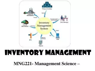
Aggregating Multiple Products in a Single Order • One of major fixed costs is transportation • Ways to lower the fixed ordering and transportation costs: • Ways to lower receiving or loading costs: • Aggregating across the products from the same supplier • Single delivery from multiple suppliers • Single delivery to multiple retailers • ASN (Advanced Shipping Notice) with EDI Microsoft。 Microsoft。 Microsoft。 14
Three computer models (L, M, H) are sold and the demand per year: M H L Example: Lot Sizing with Multiple Products • DL = 12,000; DM = 1,200; DH = 120 • Common fixed (transportation) cost, S = $4,000 • Additional product specific order cost 》sL = $1,000; sM = $1,000; sH = $1,000 Microsoft。 Microsoft。 Microsoft。 • Holding cost, h = 0.2 • Unit cost 》CL = $500; CM = $500; CH = $500 15
Delivery Options • No aggregation • Complete aggregation • Tailored aggregation • Each product is ordered separately • All products are delivered on each truck • Selected subsets of products on each truck 16
Option 1: No Aggregation Result • No aggregation • Complete aggregation • Tailored aggregation Annual total cost = $155,140 (no material cost) 17
2 DS s s s = + + + * S S = * Q L M H hC + + + * ( S n ) [( D hC / 2 n ) ( D hC / 2 n ) ( D hC / 2 n )] L L M M H H + + D hC D hC D hC * = n L L M M H H * 2 S DhC = * n 2 S Option 2: Complete Aggregation • No aggregation • Complete aggregation • Tailored aggregation • Combined fixed cost per order is given by • Let n be the number of orders placed per year. We have • Total annual cost = Annual order cost + Annual holding cost • = 18
No aggregation • Complete aggregation • Tailored aggregation • Combined fixed cost per order is given by s s s = + + + * S S L M H • Let n be the number of orders placed per year. We have • Total annual cost = Annual order cost + Annual holding cost • = + + + * ( S n ) [( D hC / 2 n ) ( D hC / 2 n ) ( D hC / 2 n )] L L M M H H + + D hC D hC D hC * = n L L M M H H * 2 S DhC = * n 2 S Option 2: Complete Aggregation 19
Option 2: Complete Aggregation Result • No aggregation • Complete aggregation • Tailored aggregation Annual order cost = 9.75×$7,000 = $68,250 Annual total cost = $68,250+$61,512+$6,151+$615=$136,528 20
Option 3: Tailored aggregation • No aggregation • Complete aggregation • Tailored aggregation A heuristic that yields an ordering policy whose cost is close to optimal. • Step 1: Identify most frequently ordered product. • Step 2: Identify frequency of other products as a multiple of the order frequency of the most frequently ordered product. • Step 3: Recalculate order frequency of most frequently ordered product. • Step 4: Identify ordering frequency of all products. 21
No aggregation • Complete aggregation • Tailored aggregation hC D L L = = = = \ = n 11 . 0 , n 3.5, n 1.1 n 11 . 0 L M H + 2 ( S s ) L • A heuristic that yields an ordering policy whose cost is close to optimal. • Step 2: Identify frequency of other products as a multiple of the order frequency of the most frequently ordered product. • Step 3: Recalculate order frequency of most frequently ordered product. • Step 4: Identify ordering frequency of all products. hCiDi = = n Max { ni } 2(S+si) i Option 3: Tailored aggregation • Step 1: Identify most frequently ordered product. 22
No aggregation • Complete aggregation • Tailored aggregation hC D L L = = = = \ = n 11 . 0 , n 3.5, n 1.1 n 11 . 0 L M H + 2 ( S s ) L A heuristic that yields an ordering policy whose cost is close to optimal. hC D = = = n M M 7 . 7 n 2.4 • Step 2: Identify frequency of other products as a multiple of the order frequency of the most frequently ordered product. M H 2 s M é ù é ù = = = = é ù m n / n 11 . 0 / 7 . 7 1 . 4 2 M M • Step 3: Recalculate order frequency of most frequently ordered product. é ù = = m 4 . 5 5 H • Step 4: Identify ordering frequency of all products. = hCiDi n= 2si Option 3: Tailored aggregation • Step 1: Identify most frequently ordered product. • Step 2: Identify frequency of other products as a multiple of the order frequency of the most frequently ordered product. 23
Step 1: Identify most frequently ordered product. • No aggregation • Complete aggregation • Tailored aggregation hC D L L = = = = \ = n 11 . 0 , n 3.5, n 1.1 n 11 . 0 L M H + 2 ( S s ) L A heuristic that yields an ordering policy whose cost is close to optimal. hC D = = = n M M 7 . 7 n 2.4 • Step 2: Identify frequency of other products as a multiple of the order frequency of the most frequently ordered product. M H 2 s M é ù é ù = = = = é ù m n / n 11 . 0 / 7 . 7 1 . 4 2 M M • Step 3: Recalculate order frequency of most frequently ordered product. é ù = = m 4 . 5 5 H å hC D m • Step 4: Identify ordering frequency of all products. i i i = n å [ ( )] + 2 S s / m i i Option 3: Tailored aggregation Derivation of n TC= order cost + holding cost • Step 2: Identify frequency of other products as a multiple of the order frequency of the most frequently ordered product. • Step 3: Recalculate order frequency of most frequently ordered product. 24
Step 1: Identify most frequently ordered product. • No aggregation • Complete aggregation • Tailored aggregation Di 2ni hC D L L = = = = \ = n 11 . 0 , n 3.5, n 1.1 n 11 . 0 L M H + 2 ( S s ) L A heuristic that yields an ordering policy whose cost is close to optimal. hC D = = = n M M 7 . 7 n 2.4 • Step 2: Identify frequency of other products as a multiple of the order frequency of the most frequently ordered product. M H 2 s M é é ù ù é ù = = = = = = é é ù ù m m n n / / n n 11 11 . . 0 0 / / 7 7 . . 7 7 1 . 4 2 M M M M • Step 3: Recalculate order frequency of most frequently ordered product. é ù = = m 4 . 5 5 H å hC D m • Step 4: Identify ordering frequency of all products. i i i = n å [ ( )] + 2 S s / m i i Option 3: Tailored aggregation Derivation of n TC= order cost+ holding cost å(hCi) ånisi + nS TC=( )+ i i å hCiDiMi å n • Step 2: Identify frequency of other products as a multiple of the order frequency of the most frequently ordered product. si i + = nS + mi 2n i • Step 3: Recalculate order frequency of most frequently ordered product. 25
Step 1: Identify most frequently ordered product. • No aggregation • Complete aggregation • Tailored aggregation hC D L L = = = = \ = n 11 . 0 , n 3.5, n 1.1 n 11 . 0 L M H + 2 ( S s ) L A heuristic that yields an ordering policy whose cost is close to optimal. å hCiDiMi si å - i =0 Þ S+ ¶ mi TC 2n2 i = 0 hC D ¶ n = = = n M M 7 . 7 n 2.4 • Step 2: Identify frequency of other products as a multiple of the order frequency of the most frequently ordered product. M H 2 s M \ é ù = = é ù m n / n 11 . 0 / 7 . 7 M M • Step 3: Recalculate order frequency of most frequently ordered product. å å hC hC D D m m • Step 4: Identify ordering frequency of all products. i i i i i i = = n n å å [ [ ( ( )] )] + + 2 2 S S s s / / m m i i i i Option 3: Tailored aggregation Derivation of n holding cost TC= order cost + å(hCi) ånisi Di + nS TC=( )+ 2ni i i å hCiDiMi å n • Step 2: Identify frequency of other products as a multiple of the order frequency of the most frequently ordered product. si i + = nS + mi 2n i • Step 3: Recalculate order frequency of most frequently ordered product. 26
Step 1: Identify most frequently ordered product. Derivation of n holding cost TC= order cost + • No aggregation • Complete aggregation • Tailored aggregation å(hCi) ånisi Di + nS TC=( )+ 2ni i i å hC D L L = = = = \ = hCiDiMi n å n 11 . 0 , n 3.5, n 1.1 n 11 . 0 L M H L si i + + = nS + 2 ( S s ) mi 2n L i A heuristic that yields an ordering policy whose cost is close to optimal. å hCiDiMi si å - i =0 Þ S+ ¶ mi TC 2n2 i = 0 hC D ¶ n = = = n M M 7 . 7 n 2.4 • Step 2: Identify frequency of other products as a multiple of the order frequency of the most frequently ordered product. M H 2 s M \ é ù é ù = = = = é ù m n / n 11 . 0 / 7 . 7 1 . 4 2 M M • Step 3: Recalculate order frequency of most frequently ordered product. é ù = = m 4 . 5 5 H å å hC hC D D m m • Step 4: Identify ordering frequency of all products. i i i i i i = = n n å å [ [ ( ( )] )] + + 2 2 S S s s / / m m i i i i Option 3: Tailored aggregation • Step 2: Identify frequency of other products as a multiple of the order frequency of the most frequently ordered product. • Step 3: Recalculate order frequency of most frequently ordered product. =11.47 Microsoft。 27
No aggregation • Complete aggregation • Tailored aggregation hC D L L = = = = \ = n 11 . 0 , n 3.5, n 1.1 n 11 . 0 L M H + 2 ( S s ) L A heuristic that yields an ordering policy whose cost is close to optimal. hC D = = = n M M 7 . 7 n 2.4 • Step 2: Identify frequency of other products as a multiple of the order frequency of the most frequently ordered product. M H 2 s M é ù é ù = = = = é ù m n / n 11 . 0 / 7 . 7 1 . 4 2 M M • Step 3: Recalculate order frequency of most frequently ordered product. é ù = = m 4 . 5 5 H å hC D m • Step 4: Identify ordering frequency of all products. i i i = n å [ ( )] + 2 S s / m i i Option 3: Tailored aggregation • Step 1: Identify most frequently ordered product. • Step 2: Identify frequency of other products as a multiple of the order frequency of the most frequently ordered product. • Step 3: Recalculate order frequency of most frequently ordered product. =11.47 nL=11.47/year, nM=11.47/2=5.74/year, nH=11.47/5=2.29/year . • Step 4: 28
Option 3: Tailored Aggregation Result • No aggregation • Complete aggregation • Tailored aggregation Annual order cost = nS+ nLsL+ sMsM + nHsH =$65,380 Annual total cost = $130,763 Complete aggregation (Annual total cost) =$136,528 29
─ A fixed cost of (S+si) is allocated to each product i, and ì ü hC D = = = The most frequently order frequency n Max n i i í ý i + 2 ( S s ) i î þ i Option 3: Tailored aggregation • No aggregation • Complete aggregation • Tailored aggregation A heuristic that yields an ordering policy whose cost is close to optimal. • Step 1: Identify most frequently ordered product. • Step 2: Identify frequency of other products as a multiple of the order frequency of the most frequently ordered product. • Step 3: Recalculate order frequency of most frequently ordered product. • Step 4: Identify ordering frequency of all products. 30
= = mi n / ni hCi Di é ù = mi mi = = ni 2si Option 3: Tailored aggregation • No aggregation • Complete aggregation • Tailored aggregation A heuristic that yields an ordering policy whose cost is close to optimal. • Step 1: Identify most frequently ordered product. • Step 2: Identify frequency of other products as a multiple of the order frequency of the most frequently ordered product. • Step 3: Recalculate order frequency of most frequently ordered product. • Step 4: Identify ordering frequency of all products. 31
å hC D m i i i = n å [ ( )] + 2 S s / m i i Option 3: Tailored aggregation • No aggregation • Complete aggregation • Tailored aggregation A heuristic that yields an ordering policy whose cost is close to optimal. • Step 1: Identify most frequently ordered product. • Step 2: Identify frequency of other products as a multiple of the order frequency of the most frequently ordered product. • Step 3: Recalculate order frequency of most frequently ordered product. • Step 4: Identify ordering frequency of all products. 32
ni=n/mi Option 3: Tailored aggregation • No aggregation • Complete aggregation • Tailored aggregation A heuristic that yields an ordering policy whose cost is close to optimal. • Step 1: Identify most frequently ordered product. • Step 2: Identify frequency of other products as a multiple of the order frequency of the most frequently ordered product. • Step 3: Recalculate order frequency of most frequently ordered product. • Step 4: Identify ordering frequency of all products. 33
S s Impact of Product Specific Order Cost ? 34
Lessons From Aggregation • Aggregation allows firm to lower lot size without increasing cost • Complete aggregation is effective if product specific fixed cost is a small fraction of joint fixed cost • Tailored aggregation is effective if product specific fixed cost is large fraction of joint fixed cost 35
Why hold inventory? • Economies of scale • Stochastic variability of supply and demand • Batch size and cycle time • Quantity discounts • Short term discounts / Trade promotions 36
Quantity Discounts • Lot size based • Volume based • Based on the quantity ordered in a single lot • All units • Marginal unit • Based on total quantity purchased over a given period • How should buyer react? How does this decision affect the supply chain in terms of lot sizes, cycle inventory, and flow time? What are appropriate discounting schemes that suppliers should offer? 37
All Unit Quantity Discounts Total Material Cost Average Cost per Unit C0 C1 C2 Quantity Purchased Order Quantity q1 q2 q3 q1 q2 q3 If an order that is at least as large as qi but smaller than qi+1 is placed, then each unit is obtained at the cost of Ci. 38
Total Cost Total Cost Lowest cost in the range Lowest cost in the range 2 DS = Qi hCi EOQi EOQi Qi D = + + TCi S hCi DCi qi qi+1 qi qi+1 Order Quantity 2 Qi Total Cost Total Cost Lowest cost in the range Lowest cost in the range qi D = + + TCi S hCi DCi 2 qi qi+1 D EOQi EOQi = + + TCi S hCi DCi+1 qi+1 2 Order Quantity Order Quantity qi qi qi+1 qi+1 Evaluate EOQ for All Unit Quantity Discounts • Evaluate EOQ for price in range qi to qi+1 , • Case 1:If qiQi < qi+1 , evaluate cost of ordering Qi • Case 2:If Qi < qi, evaluate cost of ordering qi • Case 3:If Qiqi+1 , evaluate cost of ordering qi+1 • Choose the lot size that minimizes the total cost over all price ranges. 39
2 DS = Q0 hC0 Average Cost per Unit C0 C1 C2 Quantity Purchased q1 q2 q3 Example • Assume the all unit quantity discounts • Based on the all unit quantity discounts, we have • If i = 0, evaluate Q0 as • Since Q0 > q1, we set the lost size at q1=5,000 and the total cost D = 120,000/ year S = $100/lot h = 0.2 q0=0, q1=5,000, q2=10,000 C0=$3.00, C1=$2,96, C2=$2.92 = 6,324 40
2 DS = Qi hCi Qi D = + + TCi S hCi DCi 2 Qi qi D = + + TCi S hCi DCi 2 qi qi+1 D = + + TCi S hCi DCi+1 qi+1 2 Evaluate EOQ for All Unit Quantity Discounts • Evaluate EOQ for price in range qi to qi+1 , • Case 1:If qiQi < qi+1 , evaluate cost of ordering Qi • Case 2:If Qi < qi, evaluate cost of ordering qi • Case 3:If Qiqi+1 , evaluate cost of ordering qi+1 • Choose the lot size that minimizes the total cost over all price ranges. 41
2 DS = Q0 hC0 q1 D = + + TC0 S hC1 DC1 2 q1 Example • Assume the all unit quantity discounts • Based on the all unit quantity discounts, we have • If i = 0, evaluate Q0 as • Since Q0 > q1, we set the lost size at q1=5,000 and the total cost D = 120,000/ year S = $100/lot h = 0.2 q0=0, q1=5,000, q2=10,000 C0=$3.00, C1=$2,96, C2=$2.92 = 6,324 = $359,080 42
2 DS = Q0 hC0 q1 D = + + TC0 S hC1 DC1 2 q1 Example • Assume the all unit quantity discounts • Based on the all unit quantity discounts, we have • If i = 0, evaluate Q0 as • Since Q0 > q1, we set the lost size at q1=5,000 and the total cost D = 120,000/ year S = $100/lot h = 0.2 q0=0, q1=5,000, q2=10,000 C0=$3.00, C1=$2,96, C2=$2.92 = 6,324 = $359,080 43
All Unit Quantity Discounts Total Material Cost Average Cost per Unit C0 C1 C2 Quantity Purchased Order Quantity q1 q2 q3 q1 q2 q3 If an order is placed that is at least as large as qi but smaller than qi+1, then each unit is obtained at a cost of Ci. 44
2 DS = Q0 hC0 q1 D = + + TC0 S hC1 DC1 2 q1 Example • Assume the all unit quantity discounts • Based on the all unit quantity discounts, we have • If i = 0, evaluate Q0 as • Since Q0 > q1, we set the lost size at q1=5,000 and the total cost D = 120,000/ year S = $100/lot h = 0.2 q0=0, q1=5,000, q2=10,000 C0=$3.00, C1=$2,96, C2=$2.92 = 6,324 = $359,080 45
Q1 D = + + TC1 S hC1 DC1 2 Q1 Example - Continued • For i = 1, we obtain Q1 = 6,367 Since 5,000 < Q1 <10,000 , we set the lot size at Q1 = 6,367. = $358,969 • For i = 2, we obtain Q2 = 6,410 Since Q2 < q2 , we set the lot size at q2=10,000. • Observe that the lowest total cost is for i = 2. The optimal lot size = 10,000 (at the discount price of $2.92) 46
Q1 D = $358,969 = + + TC1 S hC1 DC1 2 Q1 q2 D = + + TC2 S hC2 DC2 2 q2 Example - Continued • For i = 1, we obtain Q1 = 6,367 Since 5,000 < Q1 <10,000 , we set the lot size at Q1 = 6,367. • For i = 2, we obtain Q2 = 6,410 Since Q2 < q2 , we set the lot size at q2=10,000. = $354,520 • Observe that the lowest total cost is for i = 2. The optimal lot size = 10,000 (at the discount price of $2.92) 47
Example - Continued • For i = 1, we obtain Q1 = 6,367 Since 5,000 < Q1 <10,000 , we set the lot size at Q1 = 6,367. Q1 D = $358,969 = + + TC1 S hC1 DC1 2 Q1 • For i = 2, we obtain Q2 = 6,410 Since Q2 < q2 , we set the lot size at q2=10,000. q2 D = + + = $354,520 TC2 S hC2 DC2 2 q2 • Observe that the lowest total cost is for i = 2. The optimal lot size = 10,000 (at the discount price of $2.92) 48
q2 D = + + TC2 S hC2 DC2 2 q2 Example - Continued • For i = 1, we obtain Q1 = 6,367 Since 5,000 < Q1 <10,000 , we set the lot size at Q1 = 6,367. Q1 D = $358,969 = + + TC1 S hC1 DC1 2 Q1 • For i = 2, we obtain Q2 = 6,410 Since Q2 < q2 , we set the lot size at q2=10,000. = $354,520 • Observe that the lowest total cost is for i = 2. The optimal lot size = 10,000 (at the discount price of $2.92) 49
The Impact of All Unit Discounts on Supply Chain • In the above example • If the fixed ordering cost S = $4, • All unit quantity discounts encourage retailers to increase the size of their lots. • This also increases cycle inventory and average flow time. • The optimal order size = 6,324 when there is no discount. • The quantity discounts result in a higher order size = 10,000. • The optimal order size without discount = 1,265 • The optimal order size with all unit discounts = 10,000 50