Chapter 10 Heat Transfer
Chapter 10 Heat Transfer. Introduction to CFX. Governing Equations. Conservation Equations. Continuity. Momentum. Energy. where. Heat transfer in a fluid domain is governed by the Energy Transport Equation: The Heat Transfer Model relates to the above equation as follows


Chapter 10 Heat Transfer
E N D
Presentation Transcript
Chapter 10Heat Transfer Introduction to CFX
Governing Equations Conservation Equations Continuity Momentum Energy where
Heat transfer in a fluid domain is governed by the Energy Transport Equation: The Heat Transfer Model relates to the above equation as follows None: Energy Transport Equation not solved Isothermal: The Energy Transport Equation is not solved but a temperature is required to evaluated fluid properties (e.g. when using an Ideal Gas) Thermal Energy: An Energy Transport Equation is solved which neglects variable density effects. It is suitable for low speed liquid flow with constant specific heats. An optional viscous dissipation term can be included if viscous heating is significant. Total Energy: This models the transport of enthalpy and includes kinetic energy effects. It should be used for gas flows where the Mach number exceeds 0.2, and high speed liquid flows where viscous heating effects arise in the boundary layer, where kinetic energy effects become significant. Governing Equations Sources Viscous work Convection Conduction Transient
Governing Equations • For multicomponent flows, reacting flows and radiation modeling additional terms are included in the energy equation • Heat transfer in a solid domain is modeled using the following conduction equation Transient Conduction Source
Selecting a Heat Transfer Model • The Heat Transfer model is selected on the Domain > Fluid Models panel • Enable the Viscous Work term (Total Energy), or Viscous Dissipation term (Thermal Energy), if viscous shear in the fluid is large (e.g. lubrication or high speed compressible flows) • Enable radiation model / submodels if radiative heat transfer is significant
Radiation • Radiation effects should be accounted for when is significant compared to convective and conductive heat transfer rates • To account for radiation, Radiative Intensity Transport Equations (RTEs) are solved • Local absorption by fluid and at boundaries couples these RTEs with the energy equation • Radiation intensity is directionally and spatially dependent • Transport mechanisms for radiation intensity: • Local absorption • Out-scattering (scattering away fromthe direction) • Local emission • In-scattering (scattering into the direction)
Radiation Models • Several radiation models are available which provide approximate solutions to the RTE • Each radiation model has its assumptions, limitations, and benefits • 1) Rosseland Model (Diffusion Approximation Model) • 2) P-1 Model (Gibb’s Model/Spherical Harmonics Model) • 3) Discrete Transfer Model (DTM) (Shah Model) • 4) Monte Carlo Model (not available in the ANSYS CFD-Flo product)
Choosing a Radiation Model • The optical thickness should be determined before choosing a radiation model • Optically thin means that the fluid is transparent to the radiation at wavelengths where the heat transfer occurs • The radiation only interacts with the boundaries of the domain • Optically thick/dense means that the fluid absorbs and re-emits the radiation • For optically thick media the P1 model is a good choice • Many combustion simulations fall into this category since combustion gases tend to absorb radiation • The P1 models gives reasonable accuracy without too much computational effort
Choosing a Radiation Model • For optically thin media the Monte Carlo or Discrete Transfer models may be used • DTM can be less accurate in models with long/thin geometries • Monte Carlo uses the most computational resources, followed by DTM • Both models can be used in optically thick media, but the P1 model uses far less computational resources • Surface to Surface Model • Available for Monte Carlo and DTM • Neglects the influence of the fluid on the radiation field (only boundaries participate) • Can significantly reduce the solution time • Radiation in Solid Domains • In transparent or semi-transparent solid domains (e.g. glass) only the Monte Carlo model can be used • There is no radiation in opaque solid domains
Heat Transfer Boundary Conditions • Inlet • Static Temperature • Total Temperature • Total Enthalpy • Outlet • No details (except Radiation, see below) • Opening • Opening Temperature • Opening Static Temperature • Wall • Adiabatic • Fixed Temperature • Heat Flux • Heat Transfer Coefficient • Radiation Quantities • Local Temperature (Inlet/Outlet/Opening) • External Blackbody Temperature (Inlet/Outlet/Opening) • Opaque • Specify Emissivity and Diffuse Fraction
Domain Interfaces • GGI connections are recommended for Fluid-Solid and Solid-Solid interfaces • If radiation is modelled in one domain and not the other, set Emissivity and Diffuse Fraction values on the side which includes radiation • Set these on the boundary condition associated with the domain interface
Thin Wall Modeling • Using solid domains to model heat transfer through thin solids can present meshing problems • The thickness of the material must be resolved by the mesh • Domain interfaces can be used to model a thin material • Normal conduction only; neglects any in-plane conduction • Example: to model a baffle with heat transfer through the thickness • Create a Fluid-Fluid Domain Interface • On the Additional Interface Models tab set Mass and Momentum to No Slip Wall • This makes the interface a wall rather than an interface that fluid can pass through • Enable the Heat Transfer toggle and pick the Thin Material option • Specify a Material and Thickness • Other domain interface types (Fluid-Solid etc) can use the Thin Material option to represent coatings etc.
Thermal Contact Resistance • A Thermal Contact Resistance can be specified using the same approach as Thin Wall modeling • Just select the Thermal Contact Resistance option instead of the Thin Material option
Natural Convection • Natural convection occurswhen temperature differences in the fluid result in density variations • This is one-type of buoyancy driven flow • Flow is induced by the force of gravity acting on the density variations • As discussed in the Domains lecture, a source termSM,buoy = (r – rref) g is added to the momentum equations • The density difference (r – rref) is evaluated using either the Full Buoyancy model or the Boussinesq model • Depending on the physics the model is automatically chosen
Solution Notes • When solving heat transfer problems, make sure that you have allowed sufficient solution time for heat imbalances in all domains to become very small, particularly when Solid domains are included • Sometimes residuals reach the convergence criteria before global imbalances trend towards zero • Create Solver Monitors showing IMBALANCE levels for fluid and solid domains • View the imbalance information printed at the end of the solver output file • Use a Conservation Target when defining Solver Control in CFX-Pre
Heat Transfer Variables • The results file contains several variables related to heat transfer • Variables starting with “Wall” are only defined on walls • Temperature • This is the local fluid temperature • When plotted on a wall it is the temperature on the wall, Twall • Wall Adjacent Temperature • This is the average temperature in the control volume next to the wall • Wall Heat Transfer Coefficient, hc • By default this is based on Twall and the Wall Adjacent Temperature, not the far-field fluid temperature • Set the expert parameter “tbulk for htc” to define a far-field fluid temperature to use instead of the Wall Adjacent Temperature • Wall Heat Flux, qw • This is the total heat flux into the domain by all modes – convective and radiative (when modeled) Mesh Control Volumes qw Twall Where Tref is the Wall Adjacent Temperature or the tbulk for htc temperature if specified
Heat Transfer Variables • Heat Flux • This is the total convective heat flux into the domain • Does not include radiative heat transfer when a radiation model is used • Convective heat flux contains heat transfer due to both advection and diffusion • It can be plotted on all boundaries (inlets, outlets, walls etc) • At an inlet it would represent the energy carried with the incoming fluid relative to the fluid Reference Temperature (which is a material property, usually 25 C) • Wall Radiative Heat Flux • The net radiative energy leaving the boundary (emission minus incoming) • Heat Flux + Wall Radiative Heat Flux = Wall Heat Flux • Only applicable when radiation is modeled • Wall Irradiation Flux • The incoming radiative flux • Only applicable when radiation is modeled