The EOQ Model with Planned Backorders
The EOQ Model with Planned Backorders. Demand does not have to be satisfied immediately (from on-hand inventory). Customers are willing to wait. A penalty cost b is incurred per unit backordered per unit time. Orders are received L units of time after they are ordered. Objective.

The EOQ Model with Planned Backorders
E N D
Presentation Transcript
Demand does not have to be satisfied immediately (from on-hand inventory). • Customers are willing to wait. • A penalty cost b is incurred per unit backordered per unit time. • Orders are received L units of time after they are ordered
Objective • Minimize purchasing + ordering + holding + backordering cost
Notation • I: Average inventory level at time • B: Average number of backorders • PB: Average fraction of time there is a stock-out (stock-out probability) • B’: Average umber of units that are backordered
Q+ss L I(t) r 0 ss 2Q/D 3Q/D 4Q/D Q/D t
Let ss = r - DL, then 1. If ss > 0, I(t) > 0 and B(t) = 0, 2. If ss < - Q, I(t) = 0 and B(t) > 0 3. If -Q ss 0, then both I(t) and B(t) can be positive Only case 3 makes sense!
T: time interval between orders • T1: time interval within T during which we have positive inventory • T2: Time interval within T during which backorders are positive
Q+ss I(t) 0 t ss 2Q/D 3Q/D 4Q/D Q/D
T= Q/D • T1= (Q + ss)/D • T2= -ss/D • PB = T2/T = -ss/Q • I = (1-PB)(Q+ss)/2 = (Q+ss)2/2Q • B = PB(-ss/2) = ss2/2Q
Total Cost Let a = b/(b+h), then
Systems with Service Level Constraints • Minimize purchasing + ordering + holding cost, subject to a constraint on the probability of a stock-out.
Formulation • Minimize AD/Q + h(Q+ss)2/2Q + cD • Subject to: • PB = -ss/Q 1-ao
Since cost is increasing in ss while PB is decreasing in ss, the constraint is binding. • ss* = -Q(1- ao) • Y(Q, ss*) = AD/Q + hao2Q/2 + cD
Systems with Backorder Penalties per Occurrence • Instead of a cost b per backorder per unit time, we incur a one time cost k per backorder.
Total Cost • B’ = DPB= -Dss/Q • • Y(Q,ss) = cD + AD/Q + h(Q+ss)2/2Q -kDss/Q. • • ss* = kD/h – Q • • Y(Q,ss*)= (c+k)D + [2ADh – (kD)2]/2hQ
Two Cases • 1. +(kD)2 2ADh ss* =0 and • 2. +(kD)2 <2ADh Q* = and ss* = -
Systems with Lost Sales • No backorders are allowed • Demand that arrives when no on-hand inventory is available is considered lost • There is a penalty cost k’ (opportunity cost) for each unit of lost demand
ss’: amount of demand lost per order cycle • Q’: amount of total demand per order cycle • Q:amount of demand satisfied per order cycle = Q’-ss’ • Average number of orders per unit time = D/Q’ • Average inventory = (Q’-ss’)2/2Q’ • PB = ss’/Q’ • Average amount of demand lost per unit time = DPB= Dss’/Q’
Total cost • Y(Q’,ss’) = cD(1-ss’/Q’) + AD/Q’ + h(Q’-ss’)2/2Q’ +k’Dss’/Q’. • = cD-cDss’/Q’ + AD/Q’ + h(Q’-ss’) 2/2Q’ +k’Dss’/Q’ • = cD+ AD/Q’ + h(Q’-ss’) 2/2Q’ +(k’-c)Dss’/Q’ • The total cost has the same form as in the case with costs per backorder occurrence a similar solution approach applies.