Download
1 / 61
610 likes | 789 Vues
Chapters 1-3 - role of accounting in business. THE ROAD TRAVELED. Chapter 4-6 - how accounting information is used to plan operating activities. Chapters 7-8 - the accounting process. Chapter 9-11 recording and communication process of operating cycle activities.

E N D
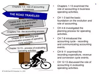
Chapters 1-3 - role of accounting in business THE ROAD TRAVELED Chapter 4-6 - how accounting information is used to plan operating activities Chapters 7-8 - the accounting process Chapter 9-11 recording and communication process of operating cycle activities Chapter 12-13 - process of evaluating operating activities • Chapters 1-13 examined the role of accounting in business operating activities. • CH 1-3 laid the basic foundation on the evolution and role of accounting. • CH 4-6 investigated the planning process for operating activities. • CH 7-8 introduced the accounting cycle - recording and communicating accounting events. • CH 9-11 examined the recording expenditure, revenue and conversion cycle events. • CH 12-13 discussed the role of accounting in evaluating operating activities.
Chapter 14 - The Time Value of Money Chapter 15 - Planning for Investing Activities Chapter 16 - Managing Human Resources and Other Non-capitalized Assets PART FIVE: PLANNING AND DECISION MAKING IN THE INVESTING AND FINANCING CYCLES
Chapter 17 - Planning for Equity Financing Activities Chapter 18 - Planning for Debt Financing Activities PART FIVE: PLANNING AND DECISION MAKING IN THE INVESTING AND FINANCING CYCLES
Begins investing and financing activities YOU ARE HERE! Foundation for second half of the course Tools for understanding capital budgeting, and human resources Discusses risk-reward relationship Chapter 14 -The Time Value of Money Tools for understanding financing decisions
CH 15 - time value of money and capital budgeting CH 16 - business considerations involving investing in human capital CH 17 - process of raising capital by issuing equity securities THE ROAD AHEAD CH 18 - process of raising capital by issuing debt securities • CH 15 uses the time value of money concepts discussed in CH 14 to examine the capital budgeting process - how companies determine whether long-term projects should be accepted or rejected. • CH 16 explores business considerations of human capital investments which are different than capital budgeting. • CH 17 and 18 explores process of raising capital necessary to run the business and make investments by raising financial resources. Chapter 3
Chapter 14 - The Time Value of Money PART FIVE: PLANNING AND DECISION MAKING IN THE INVESTING AND FINANCING CYCLES
CHAPTER 14 LEARNING OBJECTIVES L.O.1: Explain the cyclical relationship of financing, investing and operating decisions. L.O.2: Describe the distinction between return of and return on investment and the difference between rate of return and expected rate of return. L.O.3: Explain the risk-return relationship. L.O. 4: Describe the difference between simple and compound interest and how interest relates to the time value of money.
CHAPTER 14 LEARNING OBJECTIVES L.O.5: Demonstrate how to use the future value of $1 and the present value of the amount of $1 to solve problems that involve lump-sum cash flows at different points in time. L.O. 6: Demonstrate how to use the future value of an annuity and the present value of an annuity to solve problems that involve annuity cash flows.
The Management Cycle Exhibit 14.1 Operating level (coming year) Planning phase Financing Investing Strategic planning (1-5 years) Performance phase Operating Reports to Internal and External Stakeholders The management cycle is a continuous process. Operating Investing Financing Evaluation phase Performance Assessment
USE OF OPERATING PROFITS Chapter 2 • For operating activities such as replacing sold inventory, expanding inventory, extending credit to customers. • For investing activities such as acquiring new buildings and machinery, major research and development of products, and employee training programs. • For financing activities such as repayments to creditors and dividends to stockholders.
Investment X Return of investment $1,000 Sold for $1,100 a share of stock purchased for $1,000 Return on investment $100 or 10% annual return RETURN ON INVESTMENT AND RETURN OF INVESTMENT Exhibit 14.3
CALCULATING RATE OF RETURN Exhibit 14.3 Rate of = Dollar amount of return on investment Return Dollar amount of initial investment 10% = $100 $1,000
EXPECTED RATE OF RETURN Possible rates of return Likelihood they will occur Risk Expected rate of return
EXPECTED vs. ACTUAL RATE OF RETURN Before After Make the Investment Expected ROR Actual ROR Future Today
CALCULATING EXPECTED RATE OF RETURN Exhibit 14.4 Possible Possible Rate of Return Probability OutcomesReturns If Event Occursof Outcome Mother lode $1,000,000 1,000% 0.01 Full lode 150,000 150% 0.20 Baby lode 50,000 50% 0.40 No lode -100,000 -100% 0.39 Expected ROR = (.01 x 1,000% + (.2 x 150%) + (.4 x 50%) + (.39 x -100% ) = 21% Not a 21% return; rather, the possible rate of return.
ATTITUDES TOWARD RISK An investor’s attitude toward risk affects the amount of risk they may be willing to take given the decision under consideration. Risk Seeker Risk Averse
COMPARING ALTERNATIVES WITH RISK Investment A for investing $100,000 ReturnProbability Expected Return Best (11%) $11,000 .5 $5,500 Worst (10%) $10,000 .5 $5,000 $10,500 Expected rate of return on this investment equals: ($11,000/$100,000 x .5) + ($10,000/$100,000 x .5) = 10.5% Exhibit 14.5
COMPARING ALTERNATIVES WITH RISK Investment B for investing $100,000 Return Probability Expected Return Best (20%) $20,000 .5 $10,000 Worst (1%) $1,000 .5 $500 $10,500 Expected rate of return on this investment equals: ($20,000/$100,000 x .5) + (1,000/$100,000 x .5) = 10.5% Same expected return as Investment A Exhibit 14.5
RELATIVE RISK RATIO (Expected ROR - Lowest possible ROR) Expected ROR • Common-size measure ratio. • Helps rank investments according to respective risk.
COMPARING RELATIVE RISK RATIOS Investment A for investing $100,000 $10,500 - $10,000/$10,500 = 4.76% Expected ROR Worst ROR Investment B for investing $100,000 $10,500 - $1,000/$10,500 = 90.48% Worst ROR
While the opportunity for return on Investment B is greater, the range of possibilities is larger ($1,000-$20,000). This produces a greater risk. An investor must consider his or her risk tolerance and whether the capital invested is worth the risk that the return could be only 1%. PAUSE AND REFLECT Why is the relative risk ratio so high on investment B? What factors should an investor consider?
The greater the chance that the investment will return less than the expected rate, the riskier the investment. Probability of less than expected rate Amount of Risk RISK-RETURN RELATIONSHIP
RISK-RETURN RELATIONSHIP Expected ROR Price of investment Why is this relationship true?
Risk premium Expected ROR (risk-free rate) RISK-RETURN RELATIONSHIP • The riskier the investment, the less an investor is willing to pay now. An investor will demand a risk premium to make the investment. • Expected rate of return begin with the assumption called the risk-free rate of return. Risk-adjusted rate of return
RISK FACTORS • Inflation risk • Business risk • Liquidity risk There are three primary risk factors to consider that generate risk premiums for investors.
INFLATION RISK • A loaf of bread costs $1.00 on 1/1/99, but costs $1.05 on 12/31/99. • Purchasing power has declined by 5%. A return on an investment during this time would be negated, in part, by inflation. The risk that there will be a decline in purchasing power of the monetary units during the time money is invested is inflation risk.
Out of Business BUSINESS RISK The risk associated with the ability of a particular company to continue in business is a business risk.
LIQUIDITY RISK The risk that an investment cannot be quickly converted into cash is a liquidity risk.
Short-term interest rates became lower than long-term interest rates because lenders considered long-term lending riskier than short-term lending. Inflation was very volatile and could exceed the interest earned on a loan. To compensate for inflation risk, long-term interest rates were increased. Short-term loans had less risk because the loan would come due in a short period of time and the money could be loaned again at a higher rate. PAUSE AND REFLECT For many years, rates charged by banks for long-term loans such as home mortgages were lower than rates charged for short-term loans, such as car loans. In the mid-1970s, this relationship reversed and long-term loans were charged a higher interest rate than short-term loans. Why did this relationship change?
TIME VALUE OF MONEY • There is an expectation that investments generate returns over time. • This implies that a dollar today is worth more than a dollar tomorrow because it can be invested to earn a return. • This concept is known as the time value of money. A dollar invested today will be worth more tomorrow
TIME VALUE OF MONEY Assuming a 10% return on an investment: 1/1/991/1/00 $100 today is cash equivalent of $110 $100 today is worth more than $108 $100 today is worth less than $112
SIMPLE INTEREST Interest = Principal x Rate x Time Interest accrues only on the principal.
COMPOUND INTEREST Interest = (Principal + Unpaid Interest) x Rate x Time Interest accrues on the principal and any unpaid interest; interest is paid on interest or interest is earned on interest.
SIMPLE VS. COMPOUND INTEREST Compound interest Year 1 $100 Year 2 110 Year 3 121 Total $331 Simple interest Year 1 $100 Year 2 100 Year 3 100 Total $300 Assume a 3-year note, $1,000 principal at a 10% annual rate. In year 2, the interest is 10% of $1,100; in year 3, the interest is 10% of $1,210.
COMPOUNDING INTEREST Earn $700 Period 1 Earn $749 Period 2 Earn $801 Period 3 $10,000 $12,250 Invest $10,000 today at 7% Year 2 investment is $10,700 Year 3 investment is $11,449 Value at end of year 3 • Compounding is the basic underlying concept to determine the cash equivalent of cash flows that occur at different points in time. Lets see how it works on a simple investment: You invest $10,000 at 7% compounded annually. How much will your investment be worth at the end of 3 years?
COMPOUNDING INTEREST Earn $350 Period 1 Earn $362 Period 2 Earn $375 Period 3 Earn $402 Period 5 Earn $416 Period 6 Earn $388 Period 4 $10,000 $12,293 $10,350 $10,712 $11,087 $11,475 $11,877 Invest $10,000 today at 7% compounded semi-annually Value at end of year 3 More frequently than on an annual basis Lets use the previous example. If you invest $10,000 at 7% compounded semi-annually, the 3 annual periods become 6 semi-annual periods, making the effective rate of interest only 3.5%. How much will your investment be worth at the end of 3 years?
ADJUSTING COMPOUNDING INTEREST Annual Compound Rate New New Number Rate for:Rate of Periods 10.0% semi-annual 5.0% 2 periods 10.0% quarterly 2.5% 4 periods 10.0% monthly 0.83% 12 periods 10.0% daily 0.27% 365 periods More frequently than on an annual basis • To adjust an annual compound interest rate to a compound rate for more than one period, you divide the interest rate by the new number of periods in a year and multiply the periods times that same rate:
FUTURE VALUE AND PRESENT VALUE OF $1 (LUMP SUM) The concept of compounding is used to project the future value of an investment made today or the investment needed today to produce a specified sum tomorrow. Future Value of $1 Present Value of $1
FUTURE VALUE OF $1 (LUMP SUM) The future value of the amount of $1 is the amount that $1 becomes at a future date. = $1 Today $? at a future date
FUTURE VALUE OF $1 (LUMP SUM) = $? at a future date = $1,210.00 $1 Today = $1,000 @ 10% for 2 years, compounded annually By using Table 1, the future value of $1,000 can be determined by finding the intersecting point of 2 periods and 10% interest as illustrated on the next slide: $1,000 (10%, 2) = 1.2100 x $1,000, or $1,210.00
FINDING FUTURE VALUE OF $1 (LUMP SUM) IN TABLE 1 Interest Rates 10% 2 1.2100 Interest Periods
The interest rate drops from 10% to 5% and the number of periods increases from 2 periods to 4 periods. Using Table 1, the new factor is 1.2155 which produces a future value is $1,215.50. This is greater than compounding annually because interest is accruing more frequently. PAUSE AND REFLECT If interest is compounded semi-annually instead of annually, how does that change the future value problem just completed?
PRESENT VALUE OF $1 (LUMP SUM) $1 at a future date The present value of an amount of $1 is the cash equivalent today of a some specified amount of cash at some specified date in the future. = $? Today
PRESENT VALUE OF $1 (LUMP SUM) = ?$Today at 10% for 2 years, compounded annually = $1,000 $ at a future date = $1,210.00 By using Table 2 , the present value of $1,210.00 can be determined by finding the intersecting point of 2 periods and 10% interest as illustrated on the next slide. $1,210.00 (10%, 2) = .8264 x $1,210.00, or $1,000
FINDING PRESENT VALUE OF $1 (LUMP SUM) IN TABLE 2 Interest Rates 10% 2 .8264 Interest Periods
The interest rate drops from 10% to 2.5% and the number of periods increases from 2 periods to 8 periods. Using Table 2, the new factor is .8207 which producing a present value is $993.04. This is less than compounding annually because interest is accruing more frequently, meaning a smaller investment up front is needed. PAUSE AND REFLECT If interest is compounded quarterly instead of annually, how does that change the present value problem just completed?
ANNUITIES We can apply the same time value of money principles to annuities - a series of equal and periodic cash flows. Future Value of Annuity Year 1 Year 2 Year 3 Present Value of Annuity
FUTURE VALUE OF AN ANNUITY = $1 Annuity $? at a future date The future value of an annuity is the amount of money that accumulates at some future date as a result of making equal payments over equal intervals of time, earning a specified interest rate over that time period.
FUTURE VALUE OF AN ANNUITY = ?FV Annuity = $3,310 Annuity = $1,000 payments 10% for 3 years, compounded annually By using Table 3 , the future value of a $1,000 annuity can be determined by finding the intersecting point of 3 periods and 10% interest as follows as illustrated on the next slide. $1,000 (10%,3) = 3.310 x $1,000, or $3,310
FINDING FUTURE VALUE OF ANNUITY IN TABLE 3 Interest Rates 10% 3 3.310 Interest Periods