Download
1 / 70
700 likes | 794 Vues
Explore CP violation in B0s decays to measure CKM phases with relevance to unitarity triangles and quantum processes. Discover the connection to cosmology through Sakharov conditions.

E N D
≠ CP Violation in B0sJ/yf CDF (and D0) Joe Boudreau University of Pittsburgh
Vub*Vud Vtb*Vtd b Vcb*Vcd A very brief abstract of this talk first. The following topics will be developed: Vcb*Vcs CDF and D0 use B0s J/y f to measure CKM phases. We determine from this decay the quantity bs. This is in exact analogy to B factory measurement of the b, an angle of the unitarity triangle. The standard model makes very precise predictions for both angles. But other new particles & processes, lurking potentially in quantum mechanical loops such as box diagrams and penguin diagrams can change the prediction. Vub*Vus bs Vtb*Vts
The “local” connection • Studies of CPV in B0sJ/y f at the Tevatron go back to 2006, since then this has remained a “hot topic”. • Significant updates are in the works right now • From the U.K. Oxford team are major players (FarrukhAzfar and Louise Oakes); I recommend inviting them in the near future to deliver the punch line.
“Nothing is created, nothing is destroyed, everything is transformed.” e.g 2H + O H20 Lavoisier This maxim from the 18th century is wrong. Here is a recipe to produce hydrogen
A thought experiment with a box of nothing: • Take a box of nothing. • Heat it up to above the TEM, • the temperature of the electroweak • phase transition ~ 100 GeV • Cool rapidly • Open the box and you will find • something… ordinary baryonic • matter.
CKM Physics & cosmology WMap measures: The SM has all of the ingredients (Sakharov conditions) to generate the 100% Baryon Asymmetry of the Universe, but the quantity: where J is the Jarlskog Invariant Depends on quark Masses and on CP violation, thus it can be studied “in the laboratory”.
Vub*Vud Vtb*Vtd c c t t u u c u t W+ W+ W+ W+ W+ W+ W+ W+ W+ b s d s b d b s d b Vcb*Vcd The quantity “A” is the area of the“Unitarity Triangle” Vub*Vud + Vtb*Vtd + Vcb*Vcd=0
There are six unitarity triangles that can be formed, and all of them have the same area: The area of any one of these triangles quantifies how much CP violation one gets (with three generations of quark).
There are 12 observed instances of CP violation. 1. Indirect CP violation in the kaon system (eK) 2. Direct CP violation in the kaon system e’/e 3. CP Violation in the interference of mixing and decay in B0→ J/y K0. 4. CP Violation in the interference of mixing and decay in B0->h’K0 5. CP Violation in the interference of mixing and decay in B0->K+K-Ks 6. CP Violation in the interference of mixing and decay in B0->p+p- 7. CP Violation in the interference of mixing and decay in B0->D*+D- 8. CP Violation in the interference of mixing and decay in B0->f0K0s 9. CP Violation in the interference of mixing and decay in B0->yp0 10. Direct CP Violation in the decay B0K-p+ 11. Direct CP Violation in the decay B rp 12. Direct CP Violation in the decay B p+p- # 3 is important to us because: predictions are precise. there is a similarity w/ the B0sJ/y f
Very famous measurement of CP Asymmetries in B0J/y K0s |B0> | J/y K0s > |B0> Vub*Vud Vtb*Vtd b Vcb*Vcd BABAR, BELLE have used this decay to measure precisely the value of sin(2b) an angle of the bd unitarity triangle. There was a fourfold ambiguity http://ckmfitter.in2p3.fr/
Babar, Belle resolve an ambiguity in b by analyzing the decay B0J/y K0* which is BV V and measures sin(2b) and cos(2b) This involves complicated angular analysis (to be described) Phys.Rev. D71 (2005) 032005 J/y K0* Phys.Rev.Lett. 95 (2005) 091601 | P|| > |B0> | P0 > |m+m-K0sp0> |B0> |B0> | P >
|Bs0> J/y fis an almost exact analogy, except this system also contains a difference in lifetime/width) J/y f | P|| > |Bs0> | P0 > |m+m-K+K-> |Bs0> |Bs0> | P >
The decay B0sJ/yf obtains from the decay B0J/y K0* by the replacement of a d antiquark by an s antiquark b d s W W B0→J/y K0* c W d c b s s W W Bs0→J/yf c W s c We are measuring not the (bd) unitarity triangle but the (bs) unitarity triangle:
B0s→J/yf • B0s→J/yf is two particles decaying to three final states.. • Two particles: • Three final states:J/yf in an S wave CP Even • J/yf in a D wave CP Even • J/yf in a P wave CP Odd Light, CP-even, shortlived in SM Heavy, CP-odd, longlived in SM A supposedly CP even initial state decays to a supposedly CP odd final state…. like the neutral kaons Measurement needs DG≠0 but not flavor tagging. The polarization of the two vector mesons in the decay evolves with a frequency of Dms Measurement needs flavor tagging, resolution, and knowledge of Dms
Time dependence of the angular distributions: use a basis of linear polarization states of the two vector mesons { S, P, D} { P, P||, P0 } CP odd states decay to P CP even states decay to P|| ,P0 • The polarization correlation • depends on decay time. • Angular distribution of decay • products of the J/y and the f analyze the rapidly oscillating • correlation. If [H,CP] ≠ 0 Then Dms~ 17.77 ps-1. • S. Dighe, I. Dunietz, H. J. Lipkin, and J. L. Rosner, Phys. Lett. B 369, 144 (1996), • 184 hep-ph/9511363.
The measurement is a flavor-tagged analysis of time-dependent angular distributions An analysis of an oscillating polarization. This innocent expression hides a lot of richness: * CP Asymmetries through flavor tagging. * sensitivity to CP without flavor tagging. * sensitivity to both sin(2bs) and cos(2bs) simultaneously. * Width difference * Mixing Asymmetries
The flavor-tagged analysis of B0sJ/y f is a post B0s mixing analysis. * phenomenologically related * same flavor tagging technology, too. * CP violation analysis needs Dms from mixing analysis
B0s –B0s Flavor Oscillations There are two states in the B0s system, the so-called “Flavor eigenstates” They evolve according to the Schrödinger eqn and M, G Hermitian Matrices u, c u, c G: Absorptive diagrams M: Dispersive diagrams
Mass eigenstates are superpositions of flavor eigenstates governed by constants p, q: And an initially pure |B0s> evolves (oscillates) mixing probability: The magnitude of the box diagram gives the oscillation frequency Dm. The phase of the diagram determines the complex number q/p, with magnitude of very nearly 1 (in the standard model).
In general the most important components of a general purpose • detector system, for B physics, is: • tracking. • muon [+electron] id • triggering.
CDF Detector showing as seen by the B physics group. Muon chambers for triggering on the J/y→m+m- and m Identification. Strip chambers, calorimeter for electron ID Central outer tracker dE/dX and TOF system for particle ID r < 132 cm B = 1.4 T for momentum resolution.
SVX II ISL Excellent vertex resolution from three silicon subsystems: L00: 1.6 cm from the beam. 50 mm strip pitch Low mass, low M-S. For B0s mixing: SVXII can trigger on hadronic decays!!
The D0 Silicon tracker….. • surrounded by a fibre tracker at a distance 19.5 cm < r <51.5 cm • now augmented by a high-precision inner layer (“Layer 0”) • 71 (81) mm strip pitch • factor two improvement in impact • parameter resolution
Mixing is an important constraint on the Unitarity Triangle: Mixing probability Mixing occurs when a B0s decays as a B0s. Decay to a flavor specific eigenstate tags the flavor at decay: B0s Dsp; B0s Dsp p p; B0s Ds l n One of three tagging algorithms tags the flavor at production. Good triggering, full reconstruction of hadronic decays, excellent vertex resolution, and high dilution tagging are all essential for this measurement, which made news in 2006.
Δms = 18.56 ± 0.87(stat) ps-1 (D0 CONF Note 5474) (PRL 97, 242003 2006)
Two techniques for initial state “flavor tagging” • b, b quarks are always produced in pairs; • b quark always opposite b • b antiquark always opposite b • Flavor-specific decay modes (eg semileptonic decays) • of the opposite side b, or jet charge can be used to • determine the sign of the b quark on the opposite side. • The fragmentation chain produces weak • correlations between b quark flavor and the • sign of nearby pions and kaons in the • fragmentation chain • Procedure to select leading p±, K± can be optimized to obtain the highest quality tag.
Performance of the flavor tag in CDF • Each tagger returns: • A decision (B or B) • An estimate of the quality of that • decision (dilution D) • e = tag efficiency • D = 1-2w • w = mistag rate • eD2 = effective tagging efficiency
The quality of the Prediction of dilution Can be checked against the data: We reconstruct a sample Of B± decays in which one knows the sign of the B meson. We then “predict” the sign of the meson and plot the predicted dilution vs the actual dilution. Separately for B+ and B- Scale (from lepton SVT this sample; take the difference B+/B- as an uncertainty).
SST +OST: eD2 = 4.68 ± 0.54% SST: eD2 3.6% OST: eD2 1.2% Flavor Tagging Performance and Validation Each tag decision comes with an error estimate validated: 2. In the B0s mixing (SST) 1. Using B± (OST)
The measurement is a flavor-tagged analysis of time-dependent angular distributions An analysis of an oscillating polarization. This innocent expression hides a lot of richness: * CP Asymmetries through flavor tagging. * sensitivity to CP without flavor tagging. * sensitivity to both sin(2bs) and cos(2bs) simultaneously. * Width difference * Mixing Asymmetries
The analysis of B0s→J/y f can extract these physics parameters: The measurement of bs and DG are correlated; from theory one has the relation DG = 2|G12|cos(2bs) with |G12| = 0.048 ± 0.018 and A. Lenz and U. Nierste, J. High Energy Phys. 0706, 072 (2007). The exact symmetry.. … is an experimental headache.
CDF, 2506 ± 51 events .. And in D0, 1967 ± 65 total.. … but 2019 ± 73 tagged events, all tagged. …[and 3150 in 2.8 fb-1] Next, we’ll run through the CDF analysis, show what you get from flavor tagging, then show the D0 results.
Results untagged analysis Phys.Rev.Lett.100:121803,2008 Standard Model Fit (no CP violation) HQET: ct(B0s)= (1.00±0.01) ct(B0) PDG: ct(B0) = 459 ±0.027 mm
More results, untagged analysis Applying the HQET lifetime constraint:
An angular analysis can also be applied to the decay B0-> J/y K* to extract amplitudes ~ CP even / Odd fractions in the final state:
Angular fit projections B0 J/y f Angular fit projections B0 J/y K0*
A consistent picture of the CP Odd/Even fraction in B0→J/y K*, B0s→J/y f in CDF, Babar, and Belle experiments: B0 B0 B0 R. Itoh et al. Phys Rev. Lett. 98, 121801, 2007 (Belle) B. Aubert et al. PRD 76 (2007) 031102 (Babar) B0s
This plot is Feldman-Cousins confidence region in the space of the parameters 2bs and DG The likelihood for the untagged analysis has a higher degree of symmetry (dp +dwith bs - bs ) than the tagged analysis. As you will soon see
Tagged analysis: likelihood contour in the space of the parameters bs and DG One ambiguity is gone, now this one remains
Constrain strong phases d|| and d to BaBar Values (for B0J/y K* !!) Constrain ts to PDG Value for B0 Apply both constraints. using values reported in: B. Aubert et al. (BABAR Collaboration), Phys. Rev. D 71, 032005 (2005).
The standard model predictions of 2bs and DG data consistent with the CDF data at the 15% confidence level, corresponding to 1.5 Gaussian standard deviations. One dimensional Feldman-Cousins confidence intervals on 2bs ( DG treated as a nuisance parameter): 2bs [0.32, 2.82] at the 68% CL. Assuming |G12| = 0.048 ± 0.018 and the assumption of mixing-induced CP violation: 2bs [0.24,1.36] U [1.78, 2.90] at the 68% CL. If we additionally constrain the strong phases d|| and d to the results from B0 J/y K*0 decays and the Bs mean width to the world average Bd width, we find 2bs [0.40, 1.20] at 68% CL
A Feldman-Cousins confidence region in the bs-DG plane is the main result. This interval is based on p-values obtained from Toy Monte Carlo and represents regions that contain the true value of the parameters 68% (95%) of the time. arXiv:0712.2397v1 The standard model agrees with the data at the 15% CL
D0 Strategy (quite different from CDF). • Strong phases vary around the world average values ( for B0J/y K* !!) • Uncertainty taken to be ± p/5 Is this justified? Theory now estimates the • difference between the strong phases in the two decays to be < 10 o. • J. Rosner and M. Gronau, Phys.Lett.B669:321-326,2008 ) • Obtain “point estimates” in these all of these fits. • Note, D0 has a different name for the CP violation parameter: fsJ/yf = -2bs CP = CP fit, fsJ/yf floating SM = Standard model fit, fsJ/yf floating NP = New Physics fit, fsJ/yf and DG constrained by the assumption of mixing- induced CP violation.
D0 Result: arXiv:0802.2255v1
Likelihood contours for just DG and for just fs=-2bs