Download
1 / 27
270 likes | 414 Vues
SOC 206 Lecture 1. Statistics, Causation Simple Regression. Context of Discovery vs. Justification. Famous distinction by Hans Reichenbach Discovery: How do we come up with ideas Justification: How can we demonstrate that they are true. WHAT IS STATISTICS. Statistics is a language

E N D
SOC 206 Lecture 1 Statistics, Causation Simple Regression
Context of Discovery vs. Justification • Famous distinction by Hans Reichenbach • Discovery: • How do we come up with ideas • Justification: • How can we demonstrate that they are true
WHAT IS STATISTICS • Statistics is a language • Theoretical ideas can be represented • Verbally • Culture creates and reinforces power relations • Visually • Mathematically • P=f(C, e) Any language is a tool of both discovery and justification Statistics is more of a tool of justification hypothesis testing, prediction it is limited as a tool of discovery data mining, inductive statistics (factor, cluster analysis etc.) limited by its inflexibility Culture Power
Clinical vs. Statistical Prediction • Statistics allow us to process a huge amount of standardized and comparable pieces of information • Qualitative (Clinical) vs. Quantitative (Statistical) Judgment • More than a hundred studies comparing the two (Grove et al. 2001, Dawes et al. 1989) including: college admission, medical and psychiatric diagnostics, credit assessment, criminal recidivism, job performance etc. • In the overwhelming majority of the cases statistical judgment was better • Even when experts judges had more information • Even when experts were informed of the statistical prediction • Even when the statistical model was “inappropriate” but the coefficients had the right sign and unit size • Reasons: • Limited cognitive capacities • Common cognitive errors (e.g. overemphasis of recent experience, confirmation bias, ignoring base rates, human prejudice etc. • Separation of the judgment and its outcome • Self-fulfilling prophecy • Selection bias • All apply to the qualitative vs. quantitative distinction in social science methodology
Causation, Causality • Asymmetric relationship between two things one is the cause the other is the effect • John Stuart Mill’s 3 Main Criteria of Causation (System of Logic Book III. Chapter V-VIII) • Empirical Association • Statistics is strong in revealing this • Appropriate Time Order • Statistics often assumes this • Non-Spuriousness (Excluding other Forms of Causation) • Statistics uses multivariate models to establish this • Verbal representation of causality – narratives • Visual Cause (X) Effect (Y) • Mathematical Y=f(X, e)
Mathematical Description of Empirical Relationships • Y=f(X) • f= function -- e.g. Y=2X or Y=e1/ln(34X+.5X2) • The simplest function: linear – the change in Y is constant as X changes • i #of Chocolate Bars (X) Price Paid $ (Y) • 1 0 0 • 2 1 2 • 3 2 4 • 4 3 6 • 5 4 8 • 6 5 10 • Price of the chocolate bar= $2 • Price=f(count) Y=2X or Yi=2Xi
Linear Functions • i #of Chocolate Bars (X) Price Paid $ (Y) • 1 0 1 • 2 1 3 • 3 2 5 • 4 3 7 • 5 4 9 • 6 5 11 • Price of the chocolate bar= $1 entry fee + $2 per bar • Price=f(count) Y=1+2X or Yi=1+2Xi • a=intercept • b=slope • Yi=a+bXi a=1 b=2 • Y1=a+bX1 1=1+2*0 • Y2=a+bX2 3=1+2*1 • ………….. • Yn=a+bXn • Deterministic linear function
36 34 Diane 32 Steve 30 Cathy 28 Jane 26 Ben 24 22 Tom 20 18 16 14 12 10 8 6 INCOME 4 2 0 0 10 20 30 40 50 60 AGE Stochastic Linear FunctionsYi=a+bXi+ei
OLS (example) • _ _ _ _ _ _ • i Yi income Xi age Yi-Y Xi-X (Xi-X)2 (Xi-X)(Yi-Y) (Yi-Y)2 • 1 19 30 19-26= -7 30-38= -8 (-8)*(-)8= 64 (-8)*(-7)= 56 (-7)*(-7)=49 • 2 23 30 23-26= -3 30-38= -8 (-8)*(-8)= 64 (-8)*(-3)=24 (-3)*(-3)= 9 • 3 26 40 26-26= 0 40-38= 2 2 * 2 = 4 0 * 2 = 0 0 * 0 = 0 • 4 30 40 30-26= 4 40-38= 2 2 * 2 = 4 4 * 2 = 8 4 * 4 =16 • 5 27 37 27-26= 1 37-38=-1 1 * 1 = 1 1 *(-1)= -1 1 * 1 = 1 • 6 31 51 31-26= 5 51-38=13 13 * 13 =169 5 * 13= 65 5 * 5 =25 • Σ156 228 0 0 306 152 100 • Mean26 38 • b=152/306=0.4967 • Income=a+.4967*Age+e • a=? • _ _ • a=Y-bX= 26-0.4967*38 • Income=7.1254+0.4967*Age+ei • Yi=7.1254+0.4967*Xi+ ei • 7.1254 value of Y when X=0(income at age 0) • +0.4967 unit change in Y by one unit change in X(income change for each year increase in age)
Estimating Fit • How good is our model? • Our measure is the Residual Sum of Squares • observed calculated residual/error squared residual/error • iYi Pred(Yi)=a+bXi ei=Yi-Pred(Yi) ei2=ei*ei • 1 19 22.026 -3.0261 9.1573 • 2 23 22.026 .9739 0.9485 • 3 26 26.993 -.9935 0.9870 • 4 30 26.993 3.0065 9.0390 • 5 27 25.503 1.4967 2.2401 • 6 31 32.458 -1.4575 2.1243 • Σ 0 24.4962 • Is the ResSS of Σei2=24.4962 a lot or a little? • Compared to what?
36 34 Diane 32 Steve 30 Cathy 28 Jane 26 Ben 24 22 Tom 20 18 16 14 12 10 8 6 4 INCOME 2 0 0 10 20 30 40 50 60 AGE Fit • We compare Σei2=24.4962 (or about 24.5) to the amount squared error we would have made without the regression model (total error2/total sum of squares). • What if we knew only the incomes? • Our best prediction would be the mean income. • _ • Total Error2 /Total Sum of Squares= Σ(Yi-Y)2 =100 • Reduction in error/Regression Sum of Squares= • TSS- ResSS=100-24.5 • =75.5 • Proportional Reduction in Error: • 75.5/100=.755 • R2=(TSS-ResSS)/TSS • Source SS df MS Number of obs = 6 • F( 1, 4) = 12.33 Model 75.503268 1 75.503268 Prob > F = 0.0246 Residual 24.496732 4 6.12418301 R-squared = 0.7550 • Adj R-squared = 0.6938 Total 100 5 20 Root MSE = 2.4747
Outliers Bob 18 years old and making $30K added Now Tom became an outlier (like Bob) Keeping Bob but dropping Tom
Can we generalize? Intercept in the population: α Slope in the population: β Do we have a probability (random) sample? If yes, we can proceed. Are the coefficients significantly different from 0? Is α ≠0;β≠0? Is R-square significantly different from 0? Is R Both a (intercept in the sample) and b (slope in the sample) have a probability distribution and so does R-square. Suppose we take many random samples of N=6 from this population. Each time we will get an intercept and a slope. http://lstat.kuleuven.be/java We get a sampling distribution with the following characteristics: 1. It has a normal (bell) shape 2. Its expected value is the population or true value (E(a)= α; E(b)= β). 3.The standard deviation of the sampling distribution (standard error) for b for a σ2=Σεi2/N Mean Squared Error (Mean Residual Sum of Squares) where εiis the distance between the observation i and the TRUE regression line. Because we don’t know the TRUE regression line, we can only estimate εi. Our best guess is ei. So our estimate of σ2, s2= Σei2/N-2 Statistical Significance
Testing if α ≠0 t=(a- α)/s.e.(a) t=(7.124-0)/5.470=1.302 d.f=n-2=4 Testing if β ≠0 t=(b- β)/s.e.(b) t=(.497-0)/.141=3.511 d.f=n-2=4 Income000 Coef. Std. Err. t P>t [95% Conf. Interval] Age .496732 .1414697 3.51 0.025 .1039492 .8895148 _cons 7.124183 5.469958 1.30 0.263 -8.062854 22.31122 Statistical Significance of the Coefficients
Statistical Significance of the Fit • To evaluate this we use the ANalysis Of VAriance (ANOVA) table Source SS df MS Number of obs = 6 • F( 1, 4) = 12.33 Model 75.503268 1 75.503268 Prob > F = 0.0246 Residual 24.496732 4 6.12418301 R-squared = 0.7550 • Adj R-squared = 0.6938 Total 100 5 20 Root MSE = 2.4747 • We calculate the F-statistics • F regd.f., res d.f. =(RegSS/Reg. d.f.)/(ResSS/Res.d.f.) • Regd.f.= K (# of independent variables) • Res d.f.=N-k-1 • F=(75.503/1)/(24.497/(6-1-1))=12.329 df=1,4 • In a simple regression F is the squared value of the t for the slope: 3.5112=12.327(the discrepancy is due to rounding) • The F distribution is a relative of the t distribution. Both are based on the normal distribution.
Public Schools and Social Class • Verbal: • Despite the fact, that many see schools as the ultimate vehicle of social mobility, schools reproduce social inequalities by denying high quality public education from the poor. • Visual • Statistical • School quality=f(Family income, e) Family Income School Quality
Academic Performance Index (API) in California Public Schools in 2006 as a Function of the Percent of Students Receiving Subsidized Meals Variable Obs Mean Std. Dev. Min Max API13 10242 784.2502 102.2748 311 999 Source SS df MS Number of obs = 10242 F( 1, 10240) = 2933.18 Model 23852172.8 1 23852172.8 Prob > F = 0.0000 Residual 83270168.8 10240 8131.85243 R-squared = 0.2227 Adj R-squared = 0.2226 Total 107122342 10241 10460.1447 Root MSE = 90.177 API13 Coef. Std. Err. t P>t [95% Conf. Interval] MEALS -1.730451 .0319514 -54.16 0.000 -1.793082 -1.66782 _cons 885.6367 2.073267 427.17 0.000 881.5727 889.7008
Z score for X Z score for Y The slope will be different because now everything is measured in standard deviations. It will tell you that “Y will change that many standard deviations by one standard deviation change in X.” It is called the “standardized regression coefficient a.k.a. path coefficient, a.k.a. beta weight or beta coefficient. There is no intercept in a standardized regression We multiply both sides of the equation by Zxi We do that for each case 1st, 2nd …….nth. Standardized Regression and the Standardized Regression (Path) Coefficient Normal Equation • Suppose we eliminate the natural metric of the variables and turn them into Z-scores
Normal Equation • summing the equations • Dividing by n we get the average cross-products of Z-scores which are correlations. • This is the normal equation. On one side there is a correlation. On the other side path coefficients and correlations • The final normal equation • This is how you get the metric (unstandardized) slope coefficient from the path coefficient
Simple regression . correlate API13 MEALS, means (obs=10242) Variable | Mean Std. Dev. Min Max -------------+---------------------------------------------------- API13 | 784.2502 102.2748 311 999 MEALS | 58.58963 27.88903 0 100 | API13 MEALS -------------+------------------ API13 | 1.0000 MEALS | -0.4719 1.0000 b= [102.2748/27.88903] *-.4718717=-1.730451 a= 784.2502 –(-1.730451)* 58.58963= 885.6367 . regress API13 MEALS, beta Source | SS df MS Number of obs = 10242 -------------+------------------------------ ----------------------------------------------------- F( 1, 10240) = 2933.18 Model | 23852172.8 1 23852172.8 Prob > F = 0.0000 Residual | 83270168.8 10240 8131.85243 R-squared = 0.2227 -------------+------------------------------ ---------------------------------------------------- Adj R-squared = 0.2226 Total | 107122342 10241 10460.1447 Root MSE = 90.177 --------------------------------------------------------------------------------------------------------------------------------------------------- API13 | Coef. Std. Err. t P>|t| Beta -------------+------------------------------------------------------------------------------------------------------------------------------------ MEALS | -1.730451 . 0319514 -54.16 0.000 -.4718717 _cons | 885.6367 2.073267 427.17 0.000 . -----------------------------------------------------------------------------------------------------------------------------------------------
Homoscedasticy Breusch-Pagan / Cook-Weisberg test for heteroskedasticity Ho: Constant variance Variables: fitted values of API13 chi2(1) = 120.54 Prob > chi2 = 0.0000 . regress API13 MEALS, vce(hc3) beta Linear regression Number of obs = 10242 F( 1, 10240) = 3091.00 Prob > F = 0.0000 R-squared = 0.2227 Root MSE = 90.177 ----------------------------------------------------------------------------------------------------------- | Robust HC3 API13 | Coef. Std. Err. t P>|t| Beta ------------------+-------------------------------------------------------------------------------------- MEALS | -1.730451 .031125 -55.60 0.000 -.4718717 _cons | 885.6367 2.152182 411.51 0.000 . ----------------------------------------------------------------------------------------------------------