Download
1 / 25
250 likes | 449 Vues
Stratospheric Ozone Experiment. Team UNO. Team UNO. Donald Swart Christopher Barber Michael O’Leary Gregg Ridlon Robert Sheffenstein UNO Advisor Lawrence Blanchard. Objectives. Measure ozone thickness as a function of altitude using the measurable quantities of UV intensity

E N D
Stratospheric Ozone Experiment Team UNO
Team UNO • Donald Swart • Christopher Barber • Michael O’Leary • Gregg Ridlon • Robert Sheffenstein UNO Advisor • Lawrence Blanchard
Objectives • Measure ozone thickness as a function of altitude using the measurable quantities of UV intensity • Measure UVB and UVC as it is transmitted and attenuated through the stratosphere
Background • What is UltraVoilet radiation • How does UV help to detect ozone? • Absorption cross sections • Ozone measurements • Beer-Lambert’s Law
Discovery of UV • Johann W. Ritter in 1801 projected a beam of sunlight through the prism, which split the beam into the colors of the spectrum. He them put chloride in each color to see the outcome. The red caused a small change while the deep violet darkened the chloride. Ritter placed chloride in the lightless area just beyond the violet and it darkened as it were in a smoky fire. The was evidence of another wave form just barely higher than the violet of visible light. It is now known as ultraviolet or UV light.
What is UV? • Ultraviolet (UV) radiation is part of the electromagnetic spectrum from (200nm-400nm) that is emitted by the sun. • UV rays can be made artificially by passing an electric current through a gas or vapor, such as mercury vapor. • UV accounts for approximately 7% of total solar radiation • Wavelengths: • UVA - 3200 to 4000 Å • UVB - 2800 to 3200 Å • UVC - 2000 to 2800Å
Determining ozone layer thickness • Recording altitude dependent intensities • Determining relative cloumn density measurements above the payload during the accent. • Beer-Lambert Law
Beer-Lambert Law I0 is the intensity of the incident light I1 is the intensity after passing through the material l is the distance that the light travels through the material (the path length) A is the concentration of absorbing species in the material s is the absorption coefficient of the absorber. In essence, the law states that there is an exponential dependence between the transmission of light through a substance and the concentration of the substance, and also between the transmission and the length of material that the light travels through. Thus if l and α are known, the concentration of a substance can be deduced from the amount of light transmitted by it. The value of the absorption coefficient α varies between different absorbing materials and also with wavelength for a particular material.
How do we use UV measurement to determine ozone amounts? • Variation of absorbtion levels due to different wavelengths of UV • UVA is completely transmitted through ozone • UVB is partially transmitted through ozone. • UVC is totally auttenuated by ozone.
Ozone Absorption cont. “Screening” effect Ozone peak absorption between 250 and 280 nm (2500Å – 2800Å)
Absorption Cross Sections • Elements and compounds absorb certain wavelengths of light unique to each • Ozone (O3) absorbs primarily UVB and UVC • The wavelengths of light (energy) absorbed is referred to as an absorption cross section
Ozone Absorption Cross Section • Y-axis: absorption cross section in cm2/molecule • X-axis: light wavelength in nm (10Å) • Hartley band 2100Å - 3800Å • Effectively creates a light “screen” that blocks light at certain wavelengths better than others
Air mass m=sec q • Determined from the prerecorded solar zenith angles. • Expresses the path length transversed by solar radiation to reach the earth’s surface.
Measuring Ozone • Typical unit of ozone thickness is the Dobson Unit (DU) • Defined such that 1 DU is .01 mm thick at STP and has 2.687e16 molecules/cm2 • STP is temperature and pressure at Earth’s surface (avg.) 101.325 kPa, 298 K
Payload Design • Electrical System • Mechanical System • Detection Array • Power System • Thermal System
Electrical Design The photodiode signal conditioning circuit is intended to amplify the output of the photodiode to a readable analog voltage signal which is then algebraically summed and can be measured by the ADC included on the BalloonSAT board. The combined summing-amplifier circuit is built to operate on a 9Volt dual supply power source in the form of dual 9 Volt batteries. Power for the payload is controlled by a DPDT toggle Master switch, which resides on a discrete circuit board with the main fuses.
Mechanical Design The payload mechanical design will be a cube approximately 16.5 cm to a side. This size is optimum allowing sufficient space for electronics as well as the insulation. A removable construct is used to house the internal components. A shelf of foam board 10 cm by 12.5 cm with a 6.25 cm by 5cm hole in the center will hold the BalloonSAT. A lidless box of dimensions 6.25 cm by 6.25 cm and 6.25 cm tall will house the batteries and heating element. The box will be sized to fit snuggly into the BalloonSAT shelf in order to keep all components close to the heat source to maximize heat distribution by conduction and radiation.
Detection Array This system’s goal is to collect digital data of UV intensity in a specific wavelength range which will then be correlated to effective ozone coverage. The sensors’ wavelength range is 2250 Å to 3200 Å with peak sensitivity at 2800 Å. The photodiodes are arrayed evenly around the payload exterior, one per corner.
Power System Our payload will operate on four 9V, 1200 mAh batteries that are capable of operating in temperatures as low as 233K. Two batteries will power our opamp circuit, one will power the heater, and a fourth will power the BalloonSAT itself.
Thermal System The temperature control system will consist of low mass battery/resistor array that will be activated by the BalloonSAT when internal temperatures reach 283K or lower. Heat will be distributed though the payload primarily through conduction. The heating array will be placed in immediate contact with power supply for the BalloonSAT to keep the battery at an optimum operating temperature. A heat sink will be attached to the heating elements to distribute the heat to the BalloonSAT components.
Sensor Calibration We calibrated our mercury emission at Stennis Space Center using a 1000 watt quartz-halogen tungsten coiled-coil filament lamp Standard of Spectral Radiance and a .320 m spectrograph/monochromator using a diffraction grating with 600 grooves/mm blazed at 300 nm. This standard was calibrated according to NIST standards to ±2.23%. Our mercury lamp was calibrated to within ±.25Å.
Calibration cont. Using our calibrated source we were able to determine a voltage change based on our photodiodes’ exposure to a known intensity. The summed intensity of all four photodiodes was shown to be approximately .374 V when exposed to intensities of ~.008W; therefore, the average voltage change per photodiode is .094 V.
Data Analysis In essence we will correlate voltage changes to changes in the UV intensity that is detected by our photodiodes. This will provide us viable data that will be used in eq. 2 to determine the column amount of ozone. From that column amount it will be an easy step to determine the thickness of the ozone layer. Tracking the changes in UV intensity through the end of flight will also allow us to “map” the ozone density through our maximum altitude of 30km.
Expected Results The flight profile will take us up from 0 to 30km in approximately 90 minutes. As we climb in altitude we naturally expect to see in increase in UV intensity as our payload rises above greater amounts of atmosphere. The largest change should be seen at about 15km and increase as we reach our flight peak of 30km. The curve shown on this graph represents ozone density as a function of altitude; using ozone coverage estimates for the area of 31.78°N and 95.72°W provided by NOAA and taken over the last 3 years during this week we should see approximately 305 DU of ozone coverage.