Understanding User-Level and Kernel-Level Thread Management

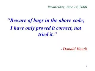
1. Wednesday, June 14, 2006 "Beware of bugs in the above code; I have only proved it correct, not tried it." - Donald Knuth

2. User level Threads • Thread switching does not require kernel mode privileges because all thread management data structures are within the user address space. Advantages • Saves overhead of two mode switches (user to kernel and kernel to user) • Scheduling can be application specific

3. User level Threads Disadvantages • When thread executes a blocking system call all threads in that process are blocked • Pure ULT systems cannot take advantage of multiprocessing

4. Kernel level Threads One to One Model: All thread management is done by kernel Scheduling is done on thread basis

5. Implementing Threads in the Kernel A threads package managed by the kernel

6. Kernel level Threads Advantages • Kernel can simultaneously schedule multiple threads from same process on multiple processors • A process with more threads can get more CPU time than a process with fewer threads

7. Kernel level Threads Disadvantages • Switching between threads is more time consuming compared to ULT

8. pthreads • POSIX standard • pthreads define API for thread creation and synchronization • Specification for behavior, not implementation • May be provided as user or kernel level library

9. Threads int count_val=0; int main(void){ int t_ret; pthread_t threadID; char cidentity[30]="Child"; char pidentity[30]="Parent"; t_ret=pthread_create(&threadID, NULL, inc_counter, (void*)cidentity); inc_counter((void*)pidentity); return 0; }

10. void* inc_counter(void* data){ char* threadname; int i; threadname = (char*)data; for(i=0;i<5; i++){ printf("%s counter is %d\n", threadname, count_val); (count_val)++; sleep(rand()%2); } pthread_exit(NULL); }

11. One possible output Parent counter is 0 Parent counter is 1 Parent counter is 2 Child counter is 3 Parent counter is 4 Child counter is 4 Parent counter is 6 Child counter is 7 Child counter is 8 Child counter is 9

12. pthread_join • joinable • Similar to zombie processes pthread_detach • If we want to let a thread exit whenever it wants to.

13. Thread Issues What if a thread calls fork()?

14. Thread Issues Thread cancellation • Concurrent search • Web browser • Asynchronous signals like Ctrl-C • Deferred Cancellation • Cancellation points • Signal Handling • Unix allows threads to specify which signals it will accept and which it will block

15. Thread Issues Private thread data

16. Scheduling Long term scheduling Short term scheduling

17. Scheduling • Long-term scheduler (or job scheduler) • Batch systems: processes are more than the resources available to execute them • selects which processes should be brought into the ready queue • Short-term scheduler (or CPU scheduler) – selects which process should be executed next and allocates CPU

18. Scheduling • Long-term scheduler (or job scheduler) • Controls degree of multiprogramming • Arrival vs departure rate • Executes less frequently • Good mix of CPU bound and I/O bound

19. Scheduling We will focus on short term scheduling • Unix and windows have no long term scheduler • New process is placed in the memory • Limits • Human nature

20. CPU Scheduling • Process • Thread

21. Alternating Sequence of CPU And I/O Bursts

22. Multiprogramming • Allow more than user at once. • Does machine now run N times slower? Not necessarily! • Key observation: users bursty. If one idle, give other resources.

24. Histogram of CPU-burst Times Based on measurements Processes tend to get more I/O bound with time

25. Scheduling Algorithm Goals

26. CPU Scheduler • Selects from among the processes in memory that are ready to execute, and allocates the CPU to one of them. • CPU scheduling decisions may take place when a process: 1. Switches from running to waiting state. 2. Switches from running to ready state. 3. Switches from waiting to ready. 4. Terminates. • Scheduling under 1 and 4 is nonpreemptive . • All other scheduling is preemptive.

27. Dispatcher • Dispatcher module gives control of the CPU to the process selected by the short-term scheduler; this involves: • switching context • switching to user mode • jumping to the proper location in the user program to restart that program • Dispatch latency – time it takes for the dispatcher to stop one process and start another running.

28. Scheduling Criteria • CPU utilization – keep the CPU as busy as possible • Throughput – # of processes that complete their execution per time unit • Turnaround time – amount of time to execute a particular process • Waiting time – amount of time a process has been waiting in the ready queue • Response time – amount of time it takes from when a request was submitted until the first response is produced, not output (for time-sharing environment)

29. Optimization Criteria • Max CPU utilization • Max throughput • Min turnaround time • Min waiting time • Min response time

30. Variance in response time

31. Small examples for demonstration purposes

32. P1 P2 P3 0 24 27 30 First-Come, First-Served (FCFS) Scheduling • Example: ProcessBurst Time P1 24 P2 3 P3 3 • Suppose that the processes arrive in the order: P1 , P2 , P3 The Gantt Chart for the schedule is:

33. P1 P2 P3 0 24 27 30 First-Come, First-Served (FCFS) Scheduling • Example: ProcessBurst Time P1 24 P2 3 P3 3 • Suppose that the processes arrive in the order: P1 , P2 , P3 The Gantt Chart for the schedule is: • Waiting time for P1 = 0; P2 = 24; P3 = 27 • Average waiting time: (0 + 24 + 27)/3 = 17

34. FCFS Scheduling (Cont.) Suppose that the processes arrive in the order P2 , P3 , P1 . • The Gantt chart for the schedule is: P2 P3 P1 0 3 6 30

35. FCFS Scheduling (Cont.) Suppose that the processes arrive in the order P2 , P3 , P1 . • The Gantt chart for the schedule is: • Waiting time for P1 = 6;P2 = 0; P3 = 3 • Average waiting time: (6 + 0 + 3)/3 = 3 • Much better than previous case. • Convoy effect short process behind long process P2 P3 P1 0 3 6 30

36. Shortest-Job-First (SJR) Scheduling • Associate with each process the length of its next CPU burst. Use these lengths to schedule the process with the shortest time. • Two schemes: • nonpreemptive – once CPU given to the process it cannot be preempted until completes its CPU burst. • Preemptive – if a new process arrives with CPU burst length less than remaining time of current executing process, preempt. This scheme is know as the Shortest-Remaining-Time-First (SRTF). • SJF is optimal – gives minimum average waiting time for a given set of processes.

37. Example of Non-Preemptive SJF Process Arrival TimeBurst Time P1 0.0 7 P2 2.0 4 P3 4.0 1 P4 5.0 4 • SJF (non-preemptive) • Average waiting time = (0 + 6 + 3 + 7)/4 - 4

38. Example of Non-Preemptive SJF Process Arrival TimeBurst Time P1 0.0 7 P2 2.0 4 P3 4.0 1 P4 5.0 4 • SJF (non-preemptive) • Average waiting time = (0 + 6 + 3 + 7)/4 = 4 P1 P3 P2 P4 0 3 7 8 12 16

39. Example of Preemptive SJF Process Arrival TimeBurst Time P1 0.0 7 P2 2.0 4 P3 4.0 1 P4 5.0 4 • SJF (preemptive) • Average waiting time = (9 + 1 + 0 +2)/4 - 3

40. Example of Preemptive SJF Process Arrival TimeBurst Time P1 0.0 7 P2 2.0 4 P3 4.0 1 P4 5.0 4 • SJF (preemptive) • Average waiting time = (9 + 1 + 0 +2)/4 = 3 P1 P2 P3 P2 P4 P1 11 16 0 2 4 5 7