Exploring Conformal Mapping for Solving 2D Problems
590 likes | 692 Vues
Dive into the powerful technique of Conformal Mapping for solving Laplace’s equation in 2D problems. Learn to map complex boundaries to simpler ones, analyze harmonic functions, and solve boundary value problems effectively.

Exploring Conformal Mapping for Solving 2D Problems
E N D
Presentation Transcript
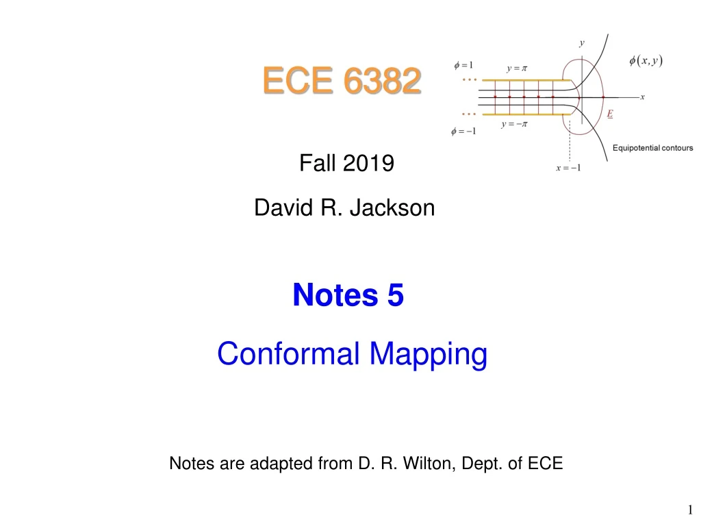
ECE 6382 Fall 2019 David R. Jackson Notes 5 Conformal Mapping Notes are adapted from D. R. Wilton, Dept. of ECE
Conformal Mapping This is a method for solving 2D problems involving Laplace’s equation. or • J. W. Brown and R. V. Churchill, Complex Variables and Applications, 9th Ed., McGraw-Hill, 2013.
Conformal Mapping (cont.) The function f (z) is assumed to be analytic in the region of interest. C A complicated boundary in the z plane is mapped into a simple one in the w plane -- for which we know how to solve the Laplace equation. z plane w plane Final Result: Desired Known
Conformal Mapping (cont.) The key to being successful with the method of conformal mapping is to find a mapping that works for your problem (i.e., it maps your problem into one the is simple enough for you to solve). • J. W. Brown and R. V. Churchill, Complex Variables and Applications, 9th Ed., McGraw-Hill, 2013. • An appendix has many basic conformal mappings. • H. Kober, Dictionary of Conformal Representations, Admiralty, Mathematical and Statistical Section, Dept. of Physical Research, 1945. • A very thorough compilation of conformal mappings.
Conformal Mapping (cont.) Theorem: If (u,v) satisfies the Laplace equation in the (u,v) plane, then (x,y) satisfies the Laplace equation in the (x,y) plane. Proof: Assume that or We want to prove that
Conformal Mapping (cont.) Using the chain rule:
Conformal Mapping (cont.) Using the chain rule:
Conformal Mapping (cont.) Use Cauchy-Riemann equations (red, blue, and black terms): satisfies Laplace’s equation.
Conformal Mapping (cont.) Recall that for any analytic function f Hence, we have (proof complete)
Conformal Mapping (cont.) Theorem that u and v are harmonic functions (revisited) Choose Note: The mapping function is arbitrary here, but it is assumed to be analytic. so that Clearly, in either case we have Hence, from our theorem, we have The functions u and v, the real and imaginary parts of an analytic function, satisfy Laplace’s equation (as we proved previously in Notes 2).
Conformal Mapping (cont.) Example (This satisfies Laplace’s equation.) Assume: (This is an analytic mapping function.) This must satisfy Laplace’s equation.
Conformal Mapping (cont.) (This satisfies Laplace’s equation.) Example Assume: (This is an analytic mapping function.) so This must satisfy Laplace’s equation.
Conformal Mapping (cont.) Theorem: If (u,v) satisfies Dirichlet or Neumann boundary conditions in the (u,v) plane, then (x,y) satisfies the same boundary conditions in the (x,y) plane. Proof: Assume that Then we immediately have that since
Conformal Mapping (cont.) Next, assume that Because of the angle-preserving (conformal) property of analytic functions, we have:
Conformal Mapping (cont.) Relation Between Charge Densities in the Two Planes so
Conformal Mapping (cont.) Hence, we have
Conformal Mapping (cont.) Theorem: The capacitance (per unit length) between two conductive objects remains unchanged between the z and w planes. Proof: (same in both planes)
Conformal Mapping (cont.) Therefore,
Conformal Mapping (cont.) Relation Between Electric Field in the Two Planes Hence Note: The electric field vector in the z plane is also rotated from that in the w plane by -argf (z0).
Example Solve for the potential inside of a coax and the capacitance per unit length of a coax.
Example (cont.) PMC PEC PEC PMC
Example (cont.) (no v dependence in ) Boundary conditions PMC PEC PEC PMC
Example (cont.) (In the final answer we use instead of r.) so or
Example (cont.) so PMC PEC PEC PMC
Example Solve for the potential inside and outside of a semi-infinite parallel-plate capacitor. Find the surface charge density on the lower surface of the top plate.
Example (cont.) The corresponding colored dots show the mapping along the top plate. Note:x reaches a maximum (x = -1) at u = 0.
Example (cont.) This is an ideal infinite parallel-plate capacitor, whose solution is simple: Note: The inside of the parallel-plate capacitor in the w plane gets mapped to the entirez plane.
Example (cont.) The solution is: For any given (x,y), these two equations have to be solved numerically to find (u,v). where
Example (cont.) The charge density in the w plane on the lower surface of the top plate is: The charge density in the z plane is:
Example (cont.) Hence we have:
Example (cont.) Rewriting in terms of x, we have: Choose negative sign (lower surface of top plate)
Example (cont.) Hence we have: or
Example (cont.) + + + + + + + Near the upper edge (on the lower surface) we then have: Note the square-root singularity at the edge!
Example Solve for the potential surrounding a metal strip, and the surface charge density on the strip. Note: The potential goes to - as .
Example (cont.) The outside of the circle gets mapped into the entirez plane. (We don’t need to consider the inside of the circle, since the points w = w0and w = 1/w0get mapped to the same z point.)
Example (cont.) Outside the circle, we have (from simple electrostatic theory): Note: To be more general, we could use Changing the constant A1changes the total charge on the strip. Changing the constant A2changes the voltage on the strip. From electrostatics (with no variation):
Example (cont.) Hence, we have: For any given (x,y), these two equations can be solved numerically to find (R,).
Example (cont.) Charge density on strip Note: Going normal to the strip in the z plane means going normal to the circle in the w plane. On the upper surface of the strip, we have:
Example (cont.) We then have
Example (cont.) Next, use so so or
Example (cont.) On the circle: so
Example (cont.) On the strip: so Hence, we have Note: The surface charge density goes to infinity as we approach the edges. This result was first derived by Maxwell!
Example (cont.) y Heresis the distance from the edge. Knife-edge singularity x The strip now has a width of w, and the total line charge density (sum of top and bottom line charge densities) is assumed to be l [C/m]. w Note: The normalization of 1/ corresponds to a unity total line charge density:
Example (cont.) Microstrip line y w h x Note: The increased current density near the edges causes increased conductor loss and susceptibility to dielectric breakdown.
Example Find the capacitance between two wires. Radii and offset: (from Churchill book) Hence, we have: • J. W. Brown and R. V. Churchill, Complex Variables and Applications, 9th Ed., McGraw-Hill, 2013.
Example (cont.) We therefore have where
Example (cont.) Symmetrical “twin lead” transmission line Scale this geometry by 1/a: x
Example (cont.) Symmetrical “twin lead” transmission line
Example (cont.) Define: