Computer Graphics Viewing
Computer Graphics Viewing. Shmuel Wimer Bar Ilan Univ., School of Engineering. Clipping Window. Viewport. World Coordinates. The clipping window is mapped into a viewport. Viewing world has its own coordinates, which may be a non-uniform scaling of world coordinates. Viewport Coordinates.

Computer Graphics Viewing
E N D
Presentation Transcript
Computer Graphics Viewing Shmuel Wimer Bar Ilan Univ., School of Engineering
Clipping Window Viewport World Coordinates The clipping window is mapped into a viewport. Viewing world has its own coordinates, which may be a non-uniform scaling of world coordinates. Viewport Coordinates
Construct World-Coordinate Scene From Modeling-Coordinate Transformations World Coordinates Convert World- Coordinates to Viewing- Coordinates Viewing Coordinates Transform Viewing-Coordinates to Normalized- Coordinates Normalized Coordinates Device Coordinates Map Normalized- Coordinates to Device-Coordinates 2D viewing transformation pipeline Modeling Coordinates
Normalization and Viewport Transformations • First approach: • Normalization and window-to-viewport transformations are combined into one operation. • Viewport range can be in [0,1] x [0,1]. • Clipping takes place in [0,1] x [0,1]. • Viewport is then mapped to display device. • Second approach: • Normalization and clipping take place before viewport transformation. • Viewport coordinates are specified in screen coordinates.
1 Normalized Viewport Clipping Window 0 1 Maintain relative size and position between clipping window and viewport.
Scaling factors: Translation factors: This can also be obtained by composing transformations:
World clipping window can first be mapped to normalized square between -1 and +1, where clipping algorithm takes place, and then transform the scene into viewport given in display coordinates.
Before Clipping After Clipping Clipping Algorithms
Cohen-Sutherland Line Clipping Algorithm • Intersection calculations are expensive. Find first lines completely inside or certainly outside clipping window. Apply intersection only to undecided lines. • Perform cheaper tests before proceeding to expensive intersection calculations.
Cohen-Sutherland Line Clipping Algorithm • Assign code to every endpoint of line segment. • Borderlines of clipping window divide the plane into two halves. • A point can be characterized by a 4-bit code according to its location in half planes. • Location bit is 0 if the point is in the positive half plane, 1 otherwise. • Code assignment involves comparisons or subtractions. • Completely inside / certainly outside tests involve only logic operations of bits.
Top bit Bottom bit Right bit Left bit 1 0 0 1 1 0 0 0 1 0 1 0 0 0 0 1 0 0 0 0 0 0 1 0 0 1 0 1 0 1 0 0 0 1 1 0 Endpoint codes are 0000 for both iff line is completely inside. If endpoint codes has 1 in same bit, line is certainly outside.
Lines that cannot be decided are intersected with window border lines. Each test clips the line and the remaining is tested again for full inclusion or certain exclusion, until remaining is either empty or fully contained. Endpoints of lines are examined against left, right, bottom and top borders (can be any order).
1 0 0 1 1 0 0 0 0 0 0 1 0 0 0 0 0 1 0 1 0 1 0 0
Liang-Barsky Line Clipping Algorithm Treat undecided lines in Cohen-Sutherland more efficiently. Define clipping window by intersections of four half-planes.
Nicholl-Lee-Nicholl Line Clipping Algorithm • Creates more regions around clipping window to avoid multiple line intersection calculations. • Performs fewer comparisons and divisions than Cohen-Sutherland and Liang-Barsky, but cannot be extended to 3D, while they can. • For complete inclusion in clipping window or certain exclusion we’ll use Cohen-Sutherland.
T R L B
LT L L LR L LB
LT L L LR L LB
T T TR T L TR L L LR LB TB LB
T T TR T L TR L L LR LB TB LB
1 1’’ 1’’ 1’ 3’’ 1’ 3’’ Clipping 3 3’ 3’ 2’ 2’’ 2’ 2’’ 2 Sutherland-Hodgman Polygon Clipping Clipping Window Efficient algorithm for clipping convex polygons. Edges are clipped against every border line of clipping window. Edges are processed successively. Allows pipelining of edge clipping of polygons, as well as pipelining of different polygons.
in in out in output: output: out out output: none in out output: The four possible outputs generated by the left clipper, depending on the relative position of pair of edge endpoints.
2 2’ 2” 3 1’ 3’ 1
The four clippers can work in parallel. • Once a pair of endpoints it output by the first clipper, the second clipper can start working. • The more edges in a polygon, the more effective parallelism is. • Processing of a new polygon can start once first clipper finished processing. • No need to wait for polygon completion.
P P∩Q Q Convex Polygon Intersection Theorem: The intersection of an L-vertex convex polygon and an M-vertex convex polygon is a convex polygon of L+M vertices at most. Proof:P∩Q is an intersection of L+M interior half planes determined by the two polygons. Intersection of convex polygons can answer the question of whether two sets of points can be separated by a line.
Theorem: The intersection of an L-vertex convex polygon and an M-vertex convex polygon can be found in θ(L+M) time. Proof: Polygons are given in cyclic order of vertices. We start from the leftmost vertex of both polygons and progress along the border of both in a left-to-right fashion, defining O(L+M) slabs. Inside a slab each polygon forms a trapezoid. The intersection of two trapezoids can be calculated in constant time.
sickle R=P∩Q P Q Another solution: The non empty intersection of two convex polygons forms a sequence of “sickles” enclosing the intersection. The border of a sickle comprises internal and external sequence of vertices originating from P and Q, which are alternating in every sickle. Let P: (p1,p2,…,pL) and Q: (q1,q2,…,qM) be counterclockwise cyclically ordered. The algorithm advances such that ∂P and ∂Q are “chasing” one another, adjusting their speeds so that they meet at every intersection.
(b) (a)
(c) (d)
case (d) case (b) case (c) case (a) farthest vertex
3D Viewing Concepts World Coordinate System Viewing Coordinate System
2D Reminder Choose viewing position, direction and orientation of the camera in the world. A clipping window is defined by the size of the aperture and the lens. Viewing by computing offers many more options which camera cannot, e.g., parallel or perspective projections, hiding parts of the scene, viewing behind obstacles, etc.
Clipping window: Selects what we want to see. Viewport: Indicates where it is to be viewed on the output device (still in world coordinates). Display window: Setting into screen coordinates. In 3D the clipping is displayed on the view plane, but clipping of the scene takes place in the space by a clipping volume. 3D transformation pipeline is similar to 2D with addition of projection transformation.
Construct World-Coordinate Scene From Modeling-Coordinate Transformations Modeling Coordinates World Coordinates Viewing Coordinates Convert World- Coordinates to Viewing- Coordinates Projection Transformation Projection Coordinates Transform Projection-Coordinates to Normalized-Coordinates Normalized Coordinates Device Coordinates Map Normalized- Coordinates to Device-Coordinates 3D Viewing Transformation Pipeline
Model is given in model (self) coordinates. Conversion to world coordinates takes place. Viewing coordinate system which defines the position and orientation of the projection plane (film plane in camera) is selected, to which scene is converted. 2D clipping window (lens of camera) is defined on the projection plane (film plane) and a 3D clipping, called view volume, is established.