Schedule

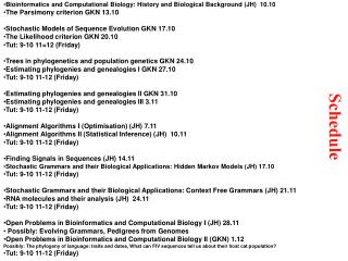
1. Bioinformatics and Computational Biology: History and Biological Background (JH) 10.10 • The Parsimony criterion GKN 13.10 • Stochastic Models of Sequence Evolution GKN 17.10 • The Likelihood criterion GKN 20.10 • Tut: 9-10 11=12 (Friday) • Trees in phylogenetics and population genetics GKN 24.10 • Estimating phylogenies and genealogies I GKN 27.10 • Tut: 9-10 11-12 (Friday) • Estimating phylogenies and genealogies II GKN 31.10 • Estimating phylogenies and genealogies III 3.11 • Tut: 9-10 11-12 (Friday) • Alignment Algorithms I (Optimisation) (JH) 7.11 • Alignment Algorithms II (Statistical Inference) (JH) 10.11 • Tut: 9-10 11-12 (Friday) • Finding Signals in Sequences (JH) 14.11 • Stochastic Grammars and their Biological Applications: Hidden Markov Models (JH) 17.10 • Tut: 9-10 11-12 (Friday) • Stochastic Grammars and their Biological Applications: Context Free Grammars (JH) 21.11 • RNA molecules and their analysis (JH) 24.11 • Tut: 9-10 11-12 (Friday) • Open Problems in Bioinformatics and Computational Biology I (JH) 28.11 • Possibly: Evolving Grammars, Pedigrees from Genomes • Open Problems in Bioinformatics and Computational Biology II (GKN) 1.12 • Possibly: The phylogeny of language: traits and dates, What can FIV sequences tell us about their host cat population? • Tut: 9-10 11-12 (Friday) Schedule

2. Bioinformatics and Computational Biology: History & Biological Background Early History up to 1953 1838 Schwann and Schleiden Cell Theory 1859 Charles Darwin publishes Origin of Species 1865 Mendel discovers basic laws of inheritance (largely ignored) 1869 Miescher Discovers DNA 1900 Mendels laws rediscovered. 1944 Avery shows DNA contains genetic information 1951 Corey & Pauling Secondary structure elements of a protein. 1953 Watson & Crick proposes DNA structure and states

3. Proteins Proteins: a string of amino acids. Often folds up in a well defined 3 dimensional structure. Has enzymatic, structural and regulatory functions.

4. DNA & RNA DNA: The Information carrier in the genetic material. Usually double helix. RNA: messenger tape from DNA to protein, regulatory, enzymatic and structural roles as well. More labile than DNA

5. An Example: t-RNA From Paul Higgs

6. Promoter Gene History up to 1953-66 1955 Sanger first protein sequence – Bovine Insulin 1957 Kendrew structure of Whale Myoglobin 1958 Crick, Goldschmidt,…. Central Dogma 1958 First quantitative method for phylogeny reconstruction (UGPMA - Sokal and Michener) 1959 Operon Models proposed (Jakob and Monod) 1966 Genetic Code Determined 1967 First RNA sequencing

7. The Central Dogma

8. The Genetic Code Genetic Code: Mapping from 3-nucleotides (codons) to amino acids (20) + stop codon. This 64-->21 mapping creates the distinction silent/replacement substitution. Substitutions Number Percent Total in all codons 549 100 Synonymous 134 25 Nonsynonymous 415 75 Missense 392 71 Nonsense 23 4 Ser Thr Glu Met Cys Leu Met Gly Gly TCA ACT GAG ATG TGT TTA ATG GGG GGA * * * * * * * ** TCG ACA GGG ATA TAT CTA ATG GGT ATA Ser Thr Gly Ile Tyr Leu Met Gly Ile

9. History 1966-80 1969-70 Temin + Baltimore Reverse Transcriptase 1970 Needleman-Wunch algorithm for pairwise alignment 1971-73 Hartigan-Fitch-Sankoff algorithm for assigning nucleotides to inner nodes on a tree. 1976/79 First viral genome – MS2/fX174 1977/8 Sharp/Roberts Introns 1979 Alternative Splicing 1980 Mitochondrial Genome (16.569bp) and the discovery of alternative codes

10. Genes, Gene Structure & Alternative Splicing • Presently estimated Gene Number: 24.000, Average Gene Size: 27 kb • The largest gene: Dystrophin 2.4 Mb - 0.6% coding – 16 hours to transcribe. • The shortest gene: tRNATYR 100% coding • Largest exon: ApoB exon 26 is 7.6 kb Smallest: <10bp • Average exon number: 9 Largest exon number: Titin 363 Smallest: 1 • Largest intron: WWOX intron 8 is 800 kb Smallest: 10s of bp • Largest polypeptide: Titin 38.138 smallest: tens – small hormones. • Intronless Genes: mitochondrial genes, many RNA genes, Interferons, Histones,.. • A challenge to automated annotation. • How widespread is it? • Is it always functional? • How does it evolve? Cartegni,L. et al.(2002) “Listening to Silence and understanding nonsense: Exonic mutations that affect splicing” Nature Reviews Genetics 3.4.285-, HMG p291-294

11. Strings and Comparing Strings 40 32 22 14 9 17 T 30 22 12 4 12 22 G 20 12 212 22 32 T 10 2 10 20 30 40 T 0 10 20 30 40 50 C T A G G Initial condition: D0,0=0. Di,j := D(s1[1:i], s2[1:j]) Di,j=min{Di-1,j-1 + d(s1[i],s2[j]), Di,j-1 + g, Di-1,j +g} Alignment:CTAGG I=2 v=5) g=10 i v Cost 17 TT-GT 1970 Needleman-Wunch algorithm for pairwise alignment for maximizing similarity 1972 Sellers-Sankoff algorithm for pairwise alignment for minimizing distance (Parsimony) 1973-5 Sankoff algorithm for multiple alignment for minimizing distance (Parsimony) and finding phylogeny simultaneously

12. History 1980-95 1981 Felsenstein Proposes algorithm to calculate probability of observed nucleotides on leaves on a tree. 1981-83 Griffiths, Hudson The Ancestral Recombination Graph. 1987/89 First biological use of Hidden Markov Model (HMM) (Lander and Green, Churchill) 1991 Thorne, Kishino and Felsenstein proposes statistical model for pairwise alignment. 1994 First biological use of stochastic context free grammar (Haussler)

13. Genealogical Structures ccagtcg Homology: The existence of a common ancestor (for instance for 2 sequences) ccggtcg cagtct Phylogeny Pedigree: Only finding common ancestors. Only one ancestor. Ancestral Recombination Graph – the ARG i. Finding common ancestors. ii. A sequence encounters Recombinations iii. A “point” ARG is a phylogeny

14. Time slices All positions have found a common ancestors on one sequence All positions have found a common ancestors Time 1 2 1 2 1 2 1 2 1 2 N 1 Population

15. 1 2 3 1 2 1 3 1 1 1 1 1 1 2 2 2 2 2 2 4 3 4 2 3 4 4 3 3 3 3 4 4 3 4 4 5 5 5 5 5 Enumerating Trees: Unrooted & valency 3 Recursion: Tn= (2n-5) Tn-1 Initialisation: T1= T2= T3=1

16. History 1995-2005 • 1995 First prokaryotic genome – H. influenzae • 1996 First unicellular eukaryotic genome – Yeast • 1998 The first multi-cellular eukaryotic genome – C.elegans • 2000 Drosophila melanogaster, Arabidopsis thaliana • 2001 Human Genome • 2002 Mouse Genome • 2005 Chimp Genome

17. The Human Genome http://www.sanger.ac.uk/HGP/ & R.Harding & HMG (2004) p 245 1 2 3 X 6 16 7 mitochondria 11 4 19 20 8 5 9 10 17 18 12 13 22 15 21 14 Y .016 45 66 72 48 51 104 3.2*109 bp 86 88 100 107 163 118 148 143 142 140 176 163 148 221 279 198 197 Myoglobin *5.000 a globin 251 b-globin (chromosome 11) 6*104 bp *20 Exon 3 Exon 1 Exon 2 3*103 bp 5’ flanking 3’ flanking *103 DNA: ATTGCCATGTCGATAATTGGACTATTTGGA 30 bp Protein: aa aa aa aa aa aa aa aa aa aa

18. Molecular Evolution and Gene Finding:Two HMMs Simple Eukaryotic Simple Prokaryotic AGTGGTACCATTTAATGCG..... Pcoding{ATG-->GTG} or AGTGGTACTATTTAGTGCG..... Pnon-coding{ATG-->GTG}

19. Three Questions for Hidden Structures. W O1 O2O3 O4O5 O6O7 O8 O9 O10 WL WR H1 H2 j L 1 i i’ j’ H3 What is the probability of the data? What is the most probable ”hidden” configuration? What is the probability of specific ”hidden” state? Training: Given a set of instances, find parameters making them probable if they were independent. HMM/Stochastic Regular Grammar SCFG - Stochastic Context Free Grammars

20. Bioinformatics and Computational Biology: History and Biological Background (JH) • The Parsimony criterion GKN • Stochastic Models of Sequence Evolution GKN • The Likelihood criterion GKN • Trees in phylogenetics and population genetics GKN • Estimating phylogenies and genealogies I GKN • Estimating phylogenies and genealogies II GKN • Estimating phylogenies and genealogies III GKN • Alignment Algorithms I (Optimisation) (JH) • Alignment Algorithms II (Statistical Inference) (JH) • Finding Signals in Sequences (JH) • Stochastic Grammars and their Biological Applications: Hidden Markov Models (JH) • Stochastic Grammars and their Biological Applications: Context Free Grammars (JH) • RNA molecules and their analysis (JH) • Open Problems in Bioinformatics and Computational Biology I (JH) • Possibly: Evolving Grammars, Pedigrees from Genomes • Open Problems in Bioinformatics and Computational Biology II (GKN) • Possibly: The phylogeny of language: traits and dates, What can FIV sequences tell us about their host cat population?