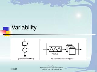
Variability Basics
Variability Basics. God does not play dice with the universe. ---Albert Einstein. Stop telling God what to do. ---Niels Bohr. Variability Makes a Difference!. Little’s Law: Consequence: Same throughput can be attained with small WIP and cycle time or with large WIP and cycle time.

Variability Basics
E N D
Presentation Transcript
Variability Basics God does not play dice with the universe. ---Albert Einstein Stop telling God what to do. ---Niels Bohr
Variability Makes a Difference! • Little’s Law: • Consequence: Same throughput can be attained with small WIP and cycle time or with large WIP and cycle time. • Difference: Variability!
Variability Views • Variability: • Any departure from uniformity • Random versus controllable variation • Randomness: • Essential reality? • Artifact of incomplete knowledge? • Management implications: robustness is key
Probabilistic Intuition • Uses of Intuition: • driving a car • throwing a ball • mastering the stock market • First Moment Effects: • Throughput increases with machine speed • Throughput increases with availability • Inventory increases with lot size • Our intuition is good for first moments
Probabilistic Intuition (cont.) • Second Moment Effects: • Which is more variable -- processing times of parts or batches? • Which are more disruptive -- long,infrequent failures or short frequent ones? • Our intuition is less secure for second moments • Misinterpretation -- e.g., regression to the mean
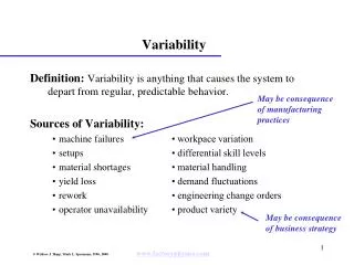
Variability • Definition: Variability is anything that causes the system to depart from regular, predictable behavior. • Sources of Variability: • setups • workpace variation • machine failures • differential skill levels • materials shortages • engineering change orders • yield loss • customer orders • rework • product differentiation • operator unavailability • material handling
Variability Classes in Factory Physics Low variability (LV) Moderate variability (MV) High variability (HV) • Effective Process Times: • actual process times are generally LV • effective process times include setups, failure outages, etc. • HV, LV, and MV are all possible in effective process times • Relation to Performance Cases: For balanced systems • MV---Practical Worst Case • LV---between Best Case and Practical Worst Case • HV---between Practical Worst Case and Worst Case ce 0 0.75 1.33
Natural Variability • Definition: variability without explicitly analyzed cause • Sources: • operator pace • material fluctuations • product type (if not explicitly considered) • product quality • Observation: natural process variability is usually in the LV category.
Down Time---Mean Effects • Definitions:
Down Time---Mean Effects (cont.) • Availability: Fraction of time machine is up • Effective Processing Time and Rate:
Down Time---Variability Effects • Effective Variability: • Conclusions: • Failures inflate mean, variance, and CV of effective process time • Mean increases proportionally with 1/A • SCV increases proportionally with mr • For constant availability (A), long infrequent outages increase CV more than short frequent ones
Down Time---Example • Data: Suppose a machine has • 15 min stroke (t0 = 15min) • 3.35 min standard deviation (s0 = 3.35min) • 12.4 hour mean time to failure(mf = 12.6 60 = 744min) • 4.133 hour repair time (mr = 4.133 60 = 248min) • Unit CV of repair time (cr = 1.0) • Natural Variability:
Down Time---Example (cont.) • Effective Variability: • Effect of Reducing MTTR: Suppose we can do frequent PM which causes mf = 1.9 hrs (= 114min), mr = 0.633 hrs (= 38min).
Setups--Mean and Variability Effects • Analysis:
Setups--Mean and Variability Effects (cont.) • Observations: • Setups increase mean and variance of processing times. • Variability reduction is one benefit of flexible machines. • However, the interaction is complex.
Setup--Example • Data: • Fast, inflexible machine--2 hr setup every 10 jobs • Slower,flexible machine--no setups • Traditional Analysis: No difference!
Setup--Example (cont.) • Factory Physics Approach: Compare mean and variance • Fast,inflexible machine--2 hr setup every 10 jobs
Setup--Example (cont.) • Slower, flexible machine--no setups • Conclusion: flexibility reduces variability.
Setup--Example (cont.) • New Machine: Consider a third machine same as previous machine with setups, but with shorter,more frequent setups • Analysis: • Conclusion: Shorter, more frequent setups induce less variability.
Other Process Variability Inflators • Sources: • operator unavailability • recycle • batching • material unavailability • et cetera, et cetera, et cetera • Effects: • inflate te • inflate ce2 • Consequences: effective process variability can be LV, MV,or HV.
Illustrating Flow Variability Low variability arrivals t High variability arrivals t
Propagation of Variability cd2(i) ca2(i+1) • Single Machine Station: where u is the station utilization given by u = rate • Multi-Machine Station: where m is the number of (identical) machines and i i+1
Propagation of Variability High Utilization Station High Process Var Low Flow Var High Flow Var Low Utilization Station High Process Var Low Flow Var Low Flow Var
Propagation of Variability High Utilization Station Low Process Var High Flow Var Low Flow Var Low Utilization Station Low Process Var High Flow Var High Flow Var
Variability Interactions • Importance of Queueing: • manufacturing plants are queueing networks • queueing and waiting time comprise majority of cycle time • System Characteristics: • Arrival process • Service process • Number of servers • Maximum queue size (blocking) • Service discipline (FCFS, LCFS, EDD, SPT, etc.) • Balking • Routing • Many more
Kendall's Classification • A/B/C A: arrival process B: service process C: number of machines M: exponential (Markovian) distribution G: completely general distribution D: constant (deterministic) distribution.
Queueing Parameters ra = the rate of arrivals in customers (jobs) per unit time (ta = 1/ra = the average time between arrivals). ca = the CV of inter-arrival times. m = the number of machines. re = the rate of the station in jobs per unit time = m/te. ce = the CV of effective process times. u = utilization of station = ra/re. Note: a station can be described with 5 parameters.
Queueing Measures • Measures: CTq = the expected waiting time spent in queue. CT = the expected time spent at the process center, i.e., queue time plus process time. WIP = the average WIP level (in jobs) at the station. WIPq = the expected WIP (in jobs) in queue. • Relationships: CT = CTq + te WIP = ra CT WIPq = ra CTq • Result: If we know CTq, we can compute WIP, WIPq, CT.
The G/G/1 Queue • Formula: • Observations: • Separate terms for variability, utilization, process time. • CTq (and other measures) increase with ca2 and ce2 • Flow variability, process variability, or both can combine to inflate queue time. • Variance causes congestion!
Variability and Cycle Time Relationships te , ce2 ra , ca2 ra , cd2
The G/G/m Queue • Analysis: • Observations: • Extremely general. • Fast and accurate. • Easily implemented in a spreadsheet (or packages like MPX).
Effects of Blocking • VUT Equation: • characterizes stations with infinite space for queueing • useful for seeing what will happen to WIP, CT without restrictions • But real world systems often constrain WIP: • physical constraints (e.g., space or spoilage) • logical constraints (e.g., kanbans) • Blocking Models: • estimate WIP and TH for given set of rates, buffer sizes • much more complex than non-blocking (open) models, often require simulation to evaluate realistic systems
Blocking Example te(1)=21 te(2)=20 B=2 M/M/1/b system has less WIP and less TH than M/M/1 system 18% less TH 90% less WIP
Attacking Variability • General Strategies: • look for long queues (Little's law) • focus on high utilization resources • consider both flow and process variability • ask “why” five times • Specific Targets: • equipment failures • setups • rework • operator pacing • anything that prevents regular arrivals and process times
Basic Variability Takeaways • Variability Measures: • CV of effective process times • CV of interarrival times • Components of Process Variability • failures • setups • many others - deflate capacity and inflate variability • long infrequent disruptions worse than short frequent ones • Consequences of Variability: • variability causes congestion (i.e., WIP/CT inflation) • variability propogates • variability and utilization interact