Interconnect Analysis for Linear Systems: Elmore Delay and Moment Matching
Chapter 4 of the organization explores linear systems, Laplace transformations, Elmore delay models, and moment matching for network analysis. Learn about poles, zeros, transfer functions, and response waveforms in time and frequency domains.

Interconnect Analysis for Linear Systems: Elmore Delay and Moment Matching
E N D
Presentation Transcript
Organization • 4.1 Linear System • 4.2 Elmore Delay • 4.3 Moment Matching and Model Order Reduction • AWE • PRIMA • 4.4 Recent development • MOR for network • Parameterized MOR
Reading Assignment for 4.1 and 4.2 • Elmore delay model (Elmore, Journal of Applied Physics, 1948 • http://eda.ee.ucla.edu/EE201A-04Spring/elmore.pdf • Elmore delay for RC tree (Rubinsteun-Penfield-Horowitz,TCAD'83 • http://eda.ee.ucla.edu/EE201A-04Spring/Elmore_TCAD.pdf
Chapter 4.1 Linear System • Laplace Transformation • Pole/residue • Basic Circuit Analysis
Laplace Transformation • Definition: time domain frequency domain Linear Circuit Time domain (t domain) Complex frequency domain (s domain) Linear equation Differential equation Laplace Transform L Inverse Transform Response waveform Response transform L-1
Frequency Domain Transfer Functionand Time Domain Impulse Response Frequency domain representation u(s) y(s) = H(s) u(s) H(s) Linear system Time domain representation u(t) h(t) Linear system The transfer function H(s) is the Laplace Transform of the impulse response h(t)
Circuit Analysis Using Laplace Transforms Time domain (t domain) Complex frequency domain (s domain) Linear Circuit Laplace Transform Differential equation Algebraic equation L Classical techniques Algebraic techniques Inverse Transform Response waveform Response transform L-1
Resonant frequencies Poles and Zeros of F(s) • Scale factor: K = bm/an • Poles: s = pk (k = 1, 2, ..., n) • Zeros: s = zk (k = 1, 2, ..., m)
pole location zero location s-plane s-plane s-plane Pole-Zero Diagrams
If poles in right-plane, waveform increases without bound as time approaches infinity Complex poles come in pairs that produce oscillatory waveforms Real poles produce exponential waveforms If poles in left-plane, waveform decays to zero as time approaches infinity If poles on j-axis, waveform neither decays nor grows Poles and Waveforms
Basic Circuit Analysis Network structures & state Natural response vN(t) (zero-input response) • Output response • Basic waveforms • Step input • Pulse input • Impulse Input • Use simple input waveforms to understand the impact of network design Forced response vF(t) (zero-state response) Input waveform & zero-states For linear circuits:
Inputs 1/T 1 0 -T/2 T/2 unit step function unit impulse function pulse function of width T 0 u(t)= 1
Time Moments of Impulse Response h(t) • Definition of moments i-th moment
Chapter 4.2 Elmore Delay • Lumped and distributed interconnect delay model • Elmore delay and distributed interconnect delay model • Elmore delay and time moments
R r r r r c c c c C Interconnect ModelLumped vs Distributed Lumped Distributed
v0u(t) v0 v0(1-eRC/T)u(t) Analysis of Simple RC Circuit zero-input response: (natural response) step-input response: match initial state: output response for step-input:
2 R4 R2 C4 C2 R1 4 1 s R3 Ri Ci C1 3 C3 i RC-Tree • The network has a single input node • All capacitors between node and ground • The network does not contain any resistive loop
2 R4 R2 C4 C2 R1 4 1 s R3 Ri Ci C1 3 C3 i RC-tree Property • Unique resistive path between the source node s and any other node i of the network path resistance Rii Example: R44=R1+R3+R4
2 R4 R2 C4 C2 R1 4 1 s R3 Ri Ci C1 3 C3 i RC-tree Property • Extended to shared path resistance Rik: Example: Ri4=R1+R3 Ri2=R1
Elmore Delay • Assuming: • Each node is initially discharged to ground • A step input is applied at time t=0 at node s • The Elmore delay at node i is: • It is an approximation: it is equivalent to first-order time constant of the network • Proven acceptable • Powerful mechanism for a quick estimate
R1 R2 RN C1 C2 CN Vin VN RC-chain (or ladder) • Special case • Shared-path resistance path resistance
R R R C C C RC-Line Delay VN Vin R=r · L/N C=c·L/N • Delay of wire is quadratic function of its length • Delay of distributed rc-line is half of lumped RC
Time Moments of Impulse Response h(t) • Definition of moments i-th moment • Note that m1 = Elmore delay when h(t) is monotone voltage response of impulse input
Definition h(t) = impulse response TD = mean of h(t) = Interpretation H(t) = output response (step process) h(t) = rate of change of H(t) T50%= median of h(t) Elmore delay approximates the median of h(t) by the mean of h(t) h(t) = impulse response H(t) = step response median of v’(t) (T50%) Elmore Delay for RC Trees
Si j path resistance Rii i input Rjk k Elmore Delay in RC Tree