Chapter 4 Indifference analysis
Chapter 4 Indifference analysis. Indifference analysis. Indifference curves. Meaning of utility. Utility is defined in 2 ways: Ordinal concept of utility Utility of each good is not measurable

Chapter 4 Indifference analysis
E N D
Presentation Transcript
Indifference analysis Indifference curves
Meaning of utility Utility is defined in 2 ways: • Ordinal concept of utility • Utility of each good is not measurable • It refers to an arbitrary assignment of numbers to rank options for the purpose of prediction or explaining human behaviour.
2. Cardinal concept of utility • Utility of each good is measurable • It refers to the inner level of satisfaction experienced by a person in the consumption process. • In HKAL exam, we will only use ordinal utility concept.
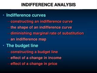
I. Basic Assumption of indifference curve appearance • Each individual chooses many goods • For each individual, some goods are scare • Economic goods are substitutable • The more a good one has, the larger the total utility, but the lower its MRS or MUV • Not all individuals choose the same goods • Individuals are consistent
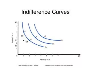
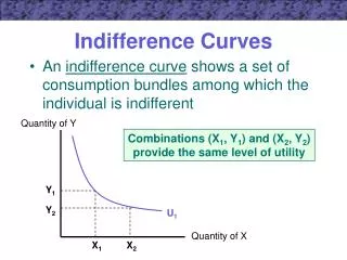
II. Meaning of indifference curve • In a two-good model, an indifference curve shows all combinations of two goods that give the same total utility to a particular individual.
Constructing an indifference curve Pears Point Oranges a b c d e f g 30 24 20 14 10 8 6 6 7 8 10 13 15 20 Combinations of pears and oranges that Clive likes the same amount as 10 pears and 13 oranges
Constructing an indifference curve a Pears Point Oranges a b c d e f g 30 24 20 14 10 8 6 6 7 8 10 13 15 20 Pears Oranges
Constructing an indifference curve a Pears Point Oranges b a b c d e f g 30 24 20 14 10 8 6 6 7 8 10 13 15 20 Pears Oranges
Constructing an indifference curve a Pears Point Oranges b a b c d e f g 30 24 20 14 10 8 6 6 7 8 10 13 15 20 c Pears d e f g Oranges
If many indifference curves are drawn together , it is called an indifference map.
An indifference map Units of good Y I1 Units of good X
An indifference map Units of good Y I2 I1 Units of good X
An indifference map Units of good Y I3 I2 I1 Units of good X
An indifference map Units of good Y I4 I3 I2 I1 Units of good X
An indifference map Units of good Y I5 I4 I3 I2 I1 Units of good X
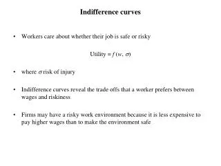
III. Characteristics of indifference • Why IC curve is downward sloping? Explain: To increase Qx, one has to decrease Qy, • Since, both entity are defined as good. To keep utility constant along the IC curve, as Qx Qy • there is a negative relationship between the consumption of good X and good Y.
Meaning of MRSxy = slope of IC curve - Y MRSxy = X • It is the maximum amount of another good that a person is willing to forgo for an extra unit of a good. • Formula: = -2 Increase in Qx by one unit, 2 Qy have to forgone to make a person satisfied with, and indifferent to both the initial and final baskets of good.
Deriving the marginal rate of substitution (MRS) a b 26 Units of good Y 6 7 Units of good X
Deriving the marginal rate of substitution (MRS) a MRS = 4 DY = 4 b 26 DX = 1 Units of good Y 6 7 Units of good X
Deriving the marginal rate of substitution (MRS) a MRS = 4 DY = 4 b 26 DX = 1 Units of good Y MRS = 1 c d DY = 1 9 DX = 1 6 7 13 14 Units of good X
IC is convex to the origin Question: MRSxy value is diminishing along the indifference curve (convex to the origin). Why? Explanation: • this is based on the postulate of diminishing marginal rate of substitution. if a person is consuming more and more of one good (Qx), he or she will be less and less willing to sacrifice the other good (Qy) for an extra unit of the good. • Value of MRS is = MUV two terms refer to the same concept
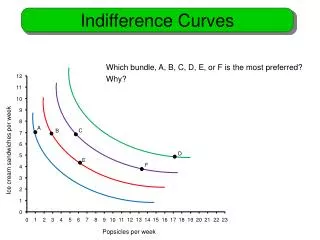
the farther the indifference curve represents higher utility level.
Question: Good Y 5 * IC3 4 3 * IC2 2 * IC 1 * Good X 0 1 2 3 4 5 • Which IC curve represents highest utility?
4. IC curve will never intersect Good Y 5 4 3 2 IC2 1 IC1 Good X 0 1 2 3 4 5 Question: • Why?
Good Y 5 * b * a 4 3 2 IC2 * c 1 IC1 * d Good X 0 1 2 3 4 5 • Assume if IC1 and IC2 now intersect, it will violate the assumption of consistency in consumption behaviour, why? Explanation: if we now make some point on the indifference curves.
Good Y 5 * b * a 4 3 2 IC2 * c 1 IC1 * d Good X 0 1 2 3 4 5 • Consider IC1, • a and c represents the combination that gives same utility level to a consumer. • Consider IC2 b and d refers to the combination that give the same utility to a consumer on a higher level than IC1.
Now if we consider only point a and b. Which one refers to higher utility? Answer: b, because it is on a higher IC. • if we consider now only point c and d, which one refers to higher utility? Answer: c since a and c are on the same IC, if c is preferred to d also, imply a is preferred to d.
but since b and d are on the same IC, it should also imply b is preferred to a. • we cannot say in the same time, b is preferred to a, but is also inferior to c. • inconsistent
Indifference analysis Budget lines
4. What is a Budget Line y BL x Definition: • It shows all combinations of two goods that are just obtainable, given an individual’s money income (nominal income, current income) and the prices of the two goods (constant). BL = PxQx+PyQy
-PX PY • Slope of the BL =
Illustrative example • given income = $360, you are require to buy only X and Y. if Px = $10 Py = $20 How many X will be bought = how many y will be bought =
y BL2 BL1 x • Draw the budget line
case A) if now I increase to $720, Px and Py remain unchanged. • new amount of X bought = • new amount of Y bought = • draw the new budget line on the same diagram Hence, the BL2 will shift out parallely, if Px and Py are constant but with I increasesreal income increase (purchasing power ) both Qx and Qy consume more
Case b) if now I decrease to $180, Px and Py remain unchanged, new amount of X bought = 18 new amount of y bought = 9 • Draw the new budget line on the same diagram. • hence, the BL will shift inward parallely, if Px and Py are constant but with I decreases purchasing power both Qx and Qy consume .
Case C) now, if I double but Px and Py double, that is: now I = $720 new Px = $20 new Py = $40 • Draw the new budget line on the same diagram. • Thus, the budget line remains unchanged with I, Px and Py change in the same proportion.
y 18 x 36 72 Case d) Assume I and Py remain the same, I = $360 Py = $20 new px = $5 new amount of X bought = 72 • Draw the new budget line on the diagram
y 36 18 9 x 36 • Hence, if I and Py remain the same BL will rotate outwards if Px falls and inwards if Px rises. Case e) Assume I and Px now are constant, new Py = $10 new amount of Y bought = 36 • Draw the new budget line.
Indifference analysis The optimal level of consumption = consumption equilibrium Postulate: budget constraint and utility maximization
Budget Line: • the preferences of a person, which is represented by an indifference map or curve • The choices available to the person, which is represented by a budget line. A person’s behaviour is limited by the choice or resources available to him/her. For a consumer, constraint on consumption is termed a budget constraint.
Consumption equilibrium • Consumption equilibrium is equal to Budget line tangent to indifference curve • budget line slope = IC curve slope • - Px / Py = - MRS
Finding the optimum consumption Units of good Y I5 I4 I3 I2 I1 O Units of good X
Finding the optimum consumption Consumption equilibrium: Budget line tangent to IC curve Units of good Y Budget line I5 I4 I3 I2 I1 O Units of good X
Finding the optimum consumption r Units of good Y I5 I4 v I3 I2 I1 O Units of good X
Finding the optimum consumption r s Units of good Y u I5 I4 v I3 I2 I1 O Units of good X
Finding the optimum consumption r s Units of good Y t u I5 I4 v I3 I2 I1 O Units of good X
Finding the optimum consumption r s Units of good Y t Y1 u I5 I4 v I3 I2 I1 O X1 Units of good X
5. Consumer equilibrium under indifference curve theory y E * BL1 x • Given a BL and an indifference map • consumer equilibrium will occur at the tangency point of the BL and the indifference curve