Download
1 / 39
390 likes | 577 Vues
Upscaling and effective properties in saturated zone transport. Wolfgang Kinzelbach IHW, ETH Zürich. Contents. Why do we need upscaling Methods Examples where we have been successful When does upscaling not work Conclusions. Dilemma in Hydrology. Point-like process information available

E N D
Upscaling and effective properties in saturated zone transport Wolfgang Kinzelbach IHW, ETH Zürich
Contents • Why do we need upscaling • Methods • Examples where we have been successful • When does upscaling not work • Conclusions
Dilemma in Hydrology • Point-like process information available • Regional statement required • Point-like information is highly variable and stochastic • Solutions to inverse problem are non-unique • Predictions based on non-unique model are doubtful
Multiscale processes • Turbulence • Catchment hydrology • Flow and transport in porous media
Possibilities for going from one scale to another • Same law – different parameter • Diffusion-Dispersion • Average transmissivity • Different law • Molecular dynamics-Gas law • Fractal geometries • Radioactive decay of mixture of radionuclides • No general law for larger scale • Singular features, non-linear processes • Small cause - big effect situations
Common Problem • Few coefficients for summing up complex subscale processes • No clear separation of scales • Way out: scale dependent coefficients
Effective parameters in transport • Ensemble mixing versus real mixing
homogen heterogen
Heterogeneity and effective parameters Cutoff Small scale Details unknown Stochastic Repetitive Modelled implicitly by parametrization Large scale Explicitly known Deterministic Singular features Modelled explicitly by flowfield Differential advection Only after a long distance (asymptotic regime) Equivalent to a diffusive process called dispersion After a shorter distance (preasymptotic) equivalent to a dual-porous medium mobile immobile
Hint for practical work: After design on the assumption of homogeneity, test your design with a set of randomly generated media An ideally designed dipole may possibly look like that:
A robust design would be the one which survives a large majority of a class of realistic random samples
Ways out • New sources of conditioning information for some processes: airborne geophysics, remote sensing from satellite of airplane platforms, environmental tracers • Simulation of small scale and Monte Carlo • Back to much simpler conceptual models • Computations only with error estimate
Model Concepts How to cope with parameter uncertainty ? Stochastic Modelling Large Scale Modelling Main interest on large observational scales Quantification of the impact of Uncertainty
Stochastic Modelling Approach Different realizations of a catchment zone Stauffer et al., WRR, 2002 Risk Assessment (question 3)
Large Scale Modelling Large Scale Predictions • Model on a „regional“ scale : 50 „small“ scale lengths • Resolution : „small“ scale length/5 • Number of unknowns
Homogenization Large Scale Flow Models with effective conductivity fine grid model large grid model
Homogenization = Asymptotic theory (scale separation between observation scale and heterogeneity scale) • Homogenization Theory • Volume averaging • Ensemble Averaging (if system ergodic)
Homogenization Large Scale Transport with effective (advection-enhanced) dispersion fine grid model large grid model
Limitations of Homogenization Problems where the scale of heterogeneities is not well separated from • Observation scale: • Process scale: velocity gradients, concentration gradients, mixing length scale
Limitations of Homogenization Natural Media = Multiscale Media with Scale Interactions, (no scale separation)
Limitations of Homogenization Question: How to model scale interactions (continuum of scales) ? pre-asymptotic system with scale dependent parameters After Schulze-Makuch et al., GW, 1999
Limitations of Homogenization process scale 1. by flow geometry 2. by mixing length scale (transient) 3. by concentration fronts Question: How to avoid artificial averaging effects?
Multiscale Modelling Improved Approach: accounts for pre-asymptotic effects Coarse Graining (Filter) Methods fine grid model coarse grid model
Multiscale Modelling: Theory Idea: Spatial filter over all length scales smaller than cut –off length scale Equivalent in Fourier Space to Attinger, J. Comp. GeoSciences,2003
Multiscale Modelling: Flow Fine scale flow model Filtered flow model
Multiscale Modelling: Flow Scale dependent mean conductivity (subscale effects) D=2: D=3: Attinger, J. Comp. GeoSciences,2003
Multiscale Modelling: Flow Statistical properties of the filtered conductivity fields
Multiscale Modelling: Transport Fine scale transport model Filtered transport model
Multiscale Modelling: Transport Scale dependent macro dispersivities: real dispersivities plus artificial mixing (centre-of-mass fluctuations)
Multiscale Modelling: Transport Scale dependent real dispersivities
Multiscale Modelling: Transport Transport Codes Model with artificial dilution Model with real dilution
Reactive Fronts Travelling fronts • Introduction of generalised spatial moment analysis (Attinger et al., MMS, 2003)
Reactive Fronts Travel time differences lead to artificial mixing by Large Scale Filtering Fine scale model Large scale Model
Reactive Fronts Local Mixing = Real Mixing Fine scale model Large scale Model
Reactive Fronts Travel time differences =nonlocal macrodispersive flux Real mixing = local real dispersive flux Dimitrova et al., AWR, 2003 Attinger et al., MMS, 2003