Download
1 / 32
370 likes | 879 Vues
Method of Soil Analysis 1.5 Geostatistics 1.5.1 Introduction 1.5.2 Using Geostatistical Methods. 1 Dec. 2004 D1 Takeshi TOKIDA. 1.5.1 Introduction. True understanding of the spatial variability in the soil map is very limited. Distinct boundary (too continuous or sudden change).

E N D
Method of Soil Analysis1.5 Geostatistics1.5.1 Introduction1.5.2 Using Geostatistical Methods 1 Dec. 2004 D1 Takeshi TOKIDA
1.5.1 Introduction • True understanding of the spatial variability in the soil map is very limited. • Distinct boundary (too continuous or sudden change). • Assumption of uniformity within a mapping unit is not necessarily valid. • Spatial and temporal variability diversify our environment. It’s Benefit! • However Soil variation can be problematic for landscape management.
1.5.1Introduction • There is a need to study surface variations in a systematic manner. • Geostatistical methods are used in a variety of disciplines. • e.g. mining, geology, and recently biological sciences also. • Numerous books have been published.
1.5.1.1 Geostatistical Investigations Geostatistics is used to… • map and identify the spatial patterns of given attributes across a landscape. • improve the efficiency of sampling networks. • identify locations in need of remediation. • Disjunctive kriging→Probability map • predict future effects in the landscape. • Random field generation→Conditioned→Predict
Analysis Appropriate data collection Objective of the study 1.5.2 Using Geostaitstical Methods1.5.2.1 Sampling • Consider the appropriate sampling methodology (see Section 1.4) The analysis of the data depend on the objective of the study and appropriate data collection.
Table 1.5-1 • If the Kolmogrov-Smirnov statistic is greater than the critical value, the hypothesis of “not being normal” is adopted. • If the distribution is completely normal, skew and kurtosis values are 0.
Table 1.5-2 ? Na values can be used to estimates B content at lower cost.
Randome function & realization • Observed data are a single realization of the random field, Z(x). Z(xα) Realization + Assumptions, i.e. stationarity Random field (Random function)
1.5.2.2 Spatial Autocorrelation • Only if a spatial correlation exists, geostatistical analysis can be used. • Fig. 1.5-1 A: No spatial correlation • Fig.1.5-1 B: spatially correlated Fig. 1.5-1
1.5.2.2.a Variogram Variogram Experimental variogram (Estimator) How to create pairs?
Variogram model Variance is undefined Var(Z) 95% Practical range
Important considerations when calculating the variogram 1 Between a lag interval, in this case 1.5 to 4.5, a wide range of actual separation distance occurs. Imprecision compared with a situation where every sampling pair has the same distance A large number of pairs are used to calculate a variogram value. It is generally accepted that 30 or more pairs are sufficient to produce a reasonable sample variogram. Fig. 1.5-3
Important considerations when calculating the variogram 2 • Width of the lag interval can affect the variance. • This is not the case. • The value for h (actual separation distance) is affected by the lag width. Fig. 1.5-4
Fig. 1.5-1 & 1.5-5 • The variograms reproduce spatial structure of simulated random fields. Fig. 1.5-1
Example of variogram Sill • Some information at the smaller scales (less than 48 m) has been lost. • For both attribute, the range is about 900 m. Sill Nugget effect Range
1.5.2.2.d Directional Variograms • Often there is a preferred orientation with higher spatial correlation in a certain direction. • For many situations, the anisotropic variogram can be transformed into an isotropic variogram by a linear transformation. Geometric anisotropy Fig. 1.5-7 Fig. 1.5-8
1.5.2.2.e Stationarity A sample at a location Impossible to determine the probability distribution at the point! The joint distribution do not depend on the location. Assumption: A stationary Z(x) has the same joint probability distribution for all locations xi and xi+h.
* Autocovariance Second-Order Stationarity 1.5-3, 1.5-6 C(0) g(h) g Sill Nugget effect C(h) h Range
If , the random field is stationary in terms of Intrinsic hypothesis. Intrinsic Stationarity(Hypothesis) No Drift Theoretical Variogram Drift? No Drift? Fig. 1.5-9
1.5.2.2.c Integral Scale 1.5-5 A measure of the distance for which the attribute is spatially correlated. 1.5-4 Autocorrelation function: normalized form of the autocovariance function
1.5.2.3 Geostatistics and Estimation • Kriging produces a best linear unbiased estimate of an atribute together with estimation variance. • Multivariate or cokriging: Superior accuracy • Powerful tool, useful in a wide variety of investigations.
1.5.2.3.a Ordinary Kriging We wish to estimate a value at xo using the data values and combining them linearly with the weiths: λi xo 1.5-7 Z* should be unbiased: 1.5-9
Derivation of equation 1.5-10 Z* should be best-linear, unbiased estimator. Our goal is to reduce as much as possible the variance of the estimation error. First, rewrite the estimation variance 0
Derivation of equation 1.5-10 Let’s rewrite the estimation variance in terms of the semivariogram. We assume intrinsic hypothesis. From the definition of the semivariogram we know:
Just substitute: Derivation of equation 1.5-10 0 1 1
Derivation of equation 1.5-10 We define an objective function φ containing a term with the Lagrange multiplier, 2β. To solve the optimization problem we set the partial derivatives to zero:
Derivation of equation 1.5-10 Ordinary Kriging system equation 1.5-10 Example:
Derivation of equation 1.5-10 Kriging Variance equation 1.5-12 Block Kriging Estimation of an average value of a spatial attribute over a region. equation 1.5-13 Average variogram values Variance equation 1.5-14 equation 1.5-15
1.5.2.3.b Validation Cross validation Little bias Estimated kriging variance is nearly equal to the actual estimation error.
1.5.2.3.c Examples Isotropic Case, Kriging Matrix. equation 1.5-18 equation 1.5-10 1.5-11 But we can’t find the values of a given attribute! λ1=0.107, λ2=0.600, λ3=0.154, λ4=0.140 Note that the weight for point 1 is less than point 4, even though the distance from the estimation site is almost the same.
Creating Maps Using Kriging Directional variogram oriented in 0°& 90° Length of each ray is equal to the range of the directional variogram. Anisotropy ratio = major axes / minor axes
Creating Maps Using Kriging Fig. 1.5-12 Based on Anisotropic variogram Fig. 1.5-13 Based on isotropic variogram