Download
1 / 20
200 likes | 233 Vues
Explore types of variation around a regression line, interpret coefficient of determination, calculate standard error of estimate, and construct prediction intervals for y values. Learn through examples and equations.

E N D
Section 9.3 Measures of Regression and Prediction Intervals
Section 9.3 Objectives • Interpret the three types of variation about a regression line • Find and interpret the coefficient of determination • Find and interpret the standard error of the estimate for a regression line • Construct and interpret a prediction interval for y
Variation About a Regression Line • Three types of variation about a regression line • Total variation • Explained variation • Unexplained variation • To find the total variation, you must first calculate • The total deviation • The explained deviation • Theunexplained deviation
Unexplained deviation Total deviation Explained deviation (xi, yi) Variation About a Regression Line Total Deviation = Explained Deviation = Unexplained Deviation = y (xi, yi) (xi, ŷi) x
Variation About a Regression Line Total variation • The sum of the squares of the differences between the y-value of each ordered pair and the mean of y. Explained variation • The sum of the squares of the differences between each predicted y-value and the mean of y. Total variation = Explained variation =
Variation About a Regression Line Unexplained variation • The sum of the squares of the differences between the y-value of each ordered pair and each corresponding predicted y-value. Unexplained variation = The sum of the explained and unexplained variation is equal to the total variation. Total variation = Explained variation + Unexplained variation
Coefficient of Determination Coefficient of determination • The ratio of the explained variation to the total variation. • Denoted by r2
Example: Coefficient of Determination The correlation coefficient for the advertising expenses and company sales data as calculated in Section 9.1 isr ≈ 0.913. Find the coefficient of determination. What does this tell you about the explained variation of the data about the regression line? About the unexplained variation? Solution: About 83.4% of the variation in the company sales can be explained by the variation in the advertising expenditures. About 16.9% of the variation is unexplained.
The Standard Error of Estimate Standard error of estimate • The standard deviation of the observed yi -values about the predicted ŷ-value for a given xi -value. • Denoted by se. • The closer the observed y-values are to the predicted y-values, the smaller the standard error of estimate will be. n is the number of ordered pairs in the data set
The Standard Error of Estimate In Words In Symbols • Make a table that includes the column heading shown. • Use the regression equation to calculate the predicted y-values. • Calculate the sum of the squares of the differences between each observed y-value and the corresponding predicted y-value. • Find the standard error of estimate.
Example: Standard Error of Estimate The regression equation for the advertising expenses and company sales data as calculated in section 9.2 isŷ = 50.729x + 104.061 Find the standard error of estimate. Solution: Use a table to calculate the sum of the squared differences of each observed y-value and the corresponding predicted y-value.
Solution: Standard Error of Estimate Σ = 635.3463 unexplained variation
Solution: Standard Error of Estimate • n = 8, Σ(yi – ŷi)2 = 635.3463 The standard error of estimate of the company sales for a specific advertising expense is about $10.29.
Prediction Intervals • Two variables have a bivariate normal distribution if for any fixed value of x, the corresponding values of y are normally distributed and for any fixed values of y, the corresponding x-values are normally distributed.
Prediction Intervals • A prediction interval can be constructed for the true value of y. • Given a linear regression equation ŷ = mx + b and x0, a specific value of x, a c-prediction intervalfor y is ŷ – E < y < ŷ + E where • The point estimate is ŷ and the margin of error is E. The probability that the prediction interval contains y is c.
Constructing a Prediction Interval for y for a Specific Value of x In Words In Symbols • Identify the number of ordered pairs in the data set n and the degrees of freedom. • Use the regression equation and the given x-value to find the point estimate ŷ. • Find the critical value tc that corresponds to the given level of confidence c. d.f. = n – 2 Use Table 5 in Appendix B.
Constructing a Prediction Interval for y for a Specific Value of x In Words In Symbols • Find the standard error of estimate se. • Find the margin of error E. • Find the left and right endpoints and form the prediction interval. Left endpoint: ŷ – E Right endpoint: ŷ + E Interval: ŷ – E < y < ŷ + E
Example: Constructing a Prediction Interval Construct a 95% prediction interval for the company sales when the advertising expenses are $2100. What can you conclude? Recall, n = 8, ŷ = 50.729x + 104.061, se = 10.290 Solution: Point estimate: ŷ = 50.729(2.1)+ 104.061 ≈ 210.592 Critical value: d.f. = n –2 = 8 – 2 = 6 tc = 2.447
Solution: Constructing a Prediction Interval Left Endpoint: ŷ – E Right Endpoint: ŷ + E 210.592 – 26.857 ≈ 183.735 210.592 + 26.857 ≈ 237.449 183.735 < y < 237.449 You can be 95% confident that when advertising expenses are $2100, the company sales will be between $183,735 and $237,449.
Section 9.3 Summary • Interpreted the three types of variation about a regression line • Found and interpreted the coefficient of determination • Found and interpreted the standard error of the estimate for a regression line • Constructed and interpreted a prediction interval for y