Download
1 / 77
770 likes | 924 Vues
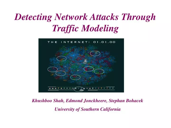
Detecting Network Attacks Through Traffic Modeling. Khushboo Shah, Edmond Jonckheere, Stephan Bohacek University of Southern California. Theme. Objective: Detect flooding attacks. Hypothesis:

E N D
Detecting Network Attacks Through Traffic Modeling Khushboo Shah, Edmond Jonckheere, Stephan Bohacek University of Southern California
Theme • Objective: • Detect flooding attacks. • Hypothesis: • The time series of non-TCP attack traffic has a statistical signature distinct from that of the time series of normal TCP traffic. • Statistical signatures being considered are: • Mutual information • Dynamic modeling prediction error
Outline • Canonical Correlation Analysis (CCA) and Mutual Information (MI) • Attack detection on different topologies using Mutual Information: • - Dumbbell topology • - Parking lot topology • - Random topology • - Transit-Stub 100 node topology • Models derived from CCA and prediction error • - State Space model using Kalman filter • - Nonlinear Auto Regressive (AR) model • Dynamic attack detection on different topologies using mean square prediction error.
Canonical Correlation Analysis Observed signal : {Y(k) : -<k<}, zero-mean random process. Past: Y-(k) = (y(k-L+1),…, y(k))T Future: Y+(k) = (y(k+1),…, y(k+L))T where L = lag One way to understand the correlation between the past and future is to examine C-+ = E(Y-Y+ T)
Canonical Correlation Analysis Observed signal : {Y(k) : -<k<}, zero-mean random process. Past: Y-(k) = (y(k-L+1),…, y(k))T Future: Y+(k) = (y(k+1),…, y(k+L))T where L = lag One way to understand the correlation between the past and future is to examine C-+ = E(Y-Y+T) Another way is to perform canonical correlation analysis:
Canonical Correlation Analysis Observed signal : {Y(k) : -<k<}, zero-mean random process. Past: Y-(k) = (y(k-L+1),…, y(k))T Future: Y+(k) = (y(k+1),…, y(k+L))T where L = lag One way to understand the correlation between the past and future is to examine C-+ = E(Y-Y+T) Another way is to perform canonical correlation analysis: Example:
Canonical Correlation Analysis Observed signal : {Y(k) : -<k<}, zero-mean random process. Past: Y-(k) = (y(k-L+1),…, y(k))T Future: Y+(k) = (y(k+1),…, y(k+L))T where L = lag One way to understand the correlation between the past and future is to examine C-+ = E(Y-Y+T) Another way is to perform canonical correlation analysis: Example:
Canonical Correlation Analysis Observed signal : {Y(k) : -<k<}, zero-mean random process. Past: Y-(k) = (y(k-L+1),…, y(k))T Future: Y+(k) = (y(k+1),…, y(k+L))T where L = lag One way to understand the correlation between the past and future is to examine C-+ = E(Y-Y+T) Another way is to perform canonical correlation analysis: Example:
Linear Canonical Correlation Analysis (LCCA) Auto-correlation of the past is: C-- = E(Y-Y-T) Auto-correlation of the future is: C++ = E(Y+Y+T) Cross correlation between the past and the future is: C-+ = E(Y-Y+T) Canonical correlation matrix between past and future: CC = C---0.5 C-+ C++-0.5
Linear Canonical Correlation Analysis (LCCA) Auto-correlation of the past is: C-- = E(Y-Y-T) Auto-correlation of the future is: C++ = E(Y+Y+T) Cross correlation between the past and the future is: C-+ = E(Y-Y+T) Canonical correlation matrix between past and future: CC = C---0.5 C-+ C++-0.5 Singular Value Decomposition of CC: CC = U V’ where U and V are orthogonal matrices, 1 1 2 … L 0 The ’s are called canonical correlation coefficients .
Linear Canonical Correlation Analysis (LCCA) Auto-correlation of the past is: C-- = E(Y-Y-T) Auto-correlation of the future is: C++ = E(Y+Y+T) Cross correlation between the past and the future is: C-+ = E(Y-Y+T) Canonical correlation matrix between past and future: CC = C---0.5 C-+ C++-0.5 Singular Value Decomposition of CC: CC = U V’ where U and V are orthogonal matrices, 1 1 2 … L 0 The ’s are called canonical correlation coefficients . Regardless of how large the lag L is, the i ’s have a breakpoint: 1 1 2 … D > > D+1… L 0 0.1 D+1 … L 0
Nonlinear Canonical Correlation Analysis (NLCCA) • Observed signal : {Y(k) : -<k<} , zero-mean random process.
Nonlinear Canonical Correlation Analysis (NLCCA) • Observed signal : {Y(k) : -<k<} , zero-mean random process. • Let (Y-(k)) be a non-linear function the past. • We restrict to be a simple polynomial:
Nonlinear Canonical Correlation Analysis (NLCCA) • Observed signal : {Y(k) : -<k<} , zero-mean random process. • Let (Y-(k)) be a non-linear function the past. • We restrict to be a simple polynomial: • Semi-NLCCA: Restrict to be a linear function of Y+(k)
Nonlinear Canonical Correlation Analysis (NLCCA) • Observed signal : {Y(k) : -<k<} , zero-mean random process. • Let (Y-(k)) be a non-linear function the past. • We restrict to be a simple polynomial: • Semi-NLCCA: Restrict to be a linear function of Y+(k) • Full-NLCCA: Restrict to be a simple polynomial of Y+(k)
Mutual Information (MI) The (Akaike) Mutual Information (MI) between the past and future vectors Y-(k) and Y+(k) is given by where the I’s are the CCCs. MI is the measure of predictability of the future signal given the past. If the CCCs are equal to zero, then MI is zero and the given time series is uncorrelated (or independent if the process is normally distributed). In contrast, if the CCCs are all one, then MI is infinite and the series is completely predictable given the knowledge of the past. Mutual information can be used to detect an attack
Outline • Canonical Correlation Analysis (CCA) and Mutual Information • Attack Detection on different topologies using mutual information. • - Dumbbell topology • - Parking lot topology • - Random topology • - Transit-Stub 100 node topology • Models derived from CCA and Prediction Error • - State Space Model using Kalman Filter • - Nonlinear Auto Regressive Model • Dynamic Attack Detection on different topologies using prediction error.
What are the observations? Packet/bytes arrivals Packet/bytes departures 0 1 simplex link • Link utilization – The number of bytesthat traverse the link in one sample period divided by the hardware bandwidth. • Packet arrivals – The number of packets that arrive at the router in one sample period.
Dumbbell Topology 7 2 8 3 Sources Destinations 0 1 9 4 1.5Mbps Node under Attack 10 5 11 6 Background traffic: FTP and HTTP traffic from the sources to the destinations. Attack traffic: CBR packets of 200 bytes are sent from the sources (2, 3, 4) to the destination (9) every 0.005 seconds (320kbps/source). Delay: 20ms Simulation run time: 30000 sec Link bandwidth: 10Mbps; Bottleneck link bandwidth: 1.5 Mbps
MI on Link Utilization for Dumbbell Topology Normal Data 1 0.9 0.8 0.7 0.6 Link Utilization 0.5 0.4 0.3 0.2 0.1 0 Attack Data 1 2 3 4 5 6 7 8 9 10 11 12 Time 4 1 x 10 0.9 0.8 0.7 0.6 Link Utilization 0.5 0.4 0.3 0.2 0.1 0 0 2000 4000 6000 8000 10000 12000 14000 16000 Time Link Utilization : No. of bytes arriving per sampling period/ hardware bandwidth
MI on Link Utilization for Dumbbell Topology Normal Data 1 Mutual Information 0.9 60 0.8 55 0.7 50 0.6 Link Utilization 45 0.5 40 0.4 Mutual Information 35 0.3 0.2 30 0.1 25 Attack 0 Non-Attack 20 Attack Data 1 2 3 4 5 6 7 8 9 10 11 12 Time 4 1 x 10 15 0.9 10 1 2 3 4 5 6 7 8 9 10 0.8 Sampling Period 0.7 0.6 Link Utilization 0.5 0.4 0.3 0.2 0.1 0 0 2000 4000 6000 8000 10000 12000 14000 16000 Time The amplitudes of the non-attack and attack signals are similar. MI is higher for the attack data than for the non-attack data. Link Utilization : No. of bytes arriving per sampling period/ hardware bandwidth
MI on Packet Arrivals for Dumbbell Topology Normal Data 500 450 400 350 300 Packet Arrivals 250 200 150 100 50 0 0 0.5 1 1.5 2 2.5 3 3.5 4 4.5 Time 4 x 10 Attack Data 500 450 400 350 300 Packet Arrivals 250 200 150 100 50 0 0 0.5 1 1.5 2 2.5 3 3.5 4 Time 4 x 10 Packet arrivals : No. of packets arriving per sampling period.
MI on Packet Arrivals for Dumbbell Topology Normal Data 500 450 Mutual Information 45 400 350 40 300 Packet Arrivals 250 35 200 30 150 Mutual Information 100 25 50 20 0 0 0.5 1 1.5 2 2.5 3 3.5 4 4.5 Non-Attack Time 4 x 10 Attack 15 Attack Data 500 450 10 1 2 3 4 5 6 7 8 9 10 Sampling Period 400 350 300 Packet Arrivals 250 200 150 100 50 0 0 0.5 1 1.5 2 2.5 3 3.5 4 Time 4 x 10 MI for the attack data is higher than that for the non-attack data, and is hence detecting the abnormality in the traffic. Packet arrivals : No. of packets arriving per sampling period.
Parking Lot Topology 0 Normal Traffic UDP Flooding Attack 8 1 2 9 10 3 Node under Attack Observed link 4 11 12 5 6 13 7 Background traffic: FTP and HTTP traffic to downstream destinations. Attack traffic: CBR packets of 200 bytes are sent to 4, at the rate of every 0.005 seconds (320kbps/source). No. of UDP connections: 15 Link bandwidth: 10Mbps Delay: 20 ms Link under investigation is : 3 – 4
MI on Link Utilization for Parking Lot Topology Normal Data 1 0.9 0.8 0.7 0.6 Link Utilization 0.5 0.4 0.3 0.2 0.1 0 0 0.5 1 1.5 2 2.5 3 Time 4 x 10 Attack Data 1 0.9 0.8 0.7 Link Utilization 0.6 0.5 0.4 0.3 0.2 0 0.5 1 1.5 2 2.5 3 Time 4 x 10 Link Utilization : No. of bytes arriving per sampling period/ hardware bandwidth
MI on Link Utilization for Parking Lot Topology Normal Data 1 0.9 Mutual Information 0.8 12 Non-Attack 0.7 Attack 0.6 11 Link Utilization 0.5 10 0.4 0.3 9 Mutual Information 0.2 0.1 8 0 0 0.5 1 1.5 2 2.5 3 7 Time 4 x 10 Attack Data 1 6 0.9 5 1 2 3 4 5 6 7 8 9 10 0.8 Sampling Period 0.7 Link Utilization 0.6 0.5 0.4 0.3 0.2 0 0.5 1 1.5 2 2.5 3 Time 4 x 10 Both time series appear to be similar. But there is a clear difference in MI. MI is higher in the case of attack data. Link Utilization : No. of bytes arriving per sampling period/ hardware bandwidth
MI on Packet Arrivals for Parking Lot Topology Normal Data 1600 1400 Mutual Information 40 1200 Attack Non-Attack 1000 35 Packet Arrivals 800 30 600 25 Mutual Information 400 20 200 0 15 1 1.5 2 2.5 3 3.5 4 Time 4 x 10 Attack Data 10 2000 1800 5 1 2 3 4 5 6 7 8 9 10 1600 Sampling Period 1400 1200 Packet Arrivals 1000 800 600 400 200 0 0 1 2 3 4 5 6 Time 4 x 10 Both time-series look similar. But the statistics reveals the anomaly in the traffic. Packet arrivals : No. of packets arriving per sampling period.
What are the observations? Mutual Information Mutual Information 60 45 55 40 50 35 45 40 Mutual Information 30 Mutual Information 35 25 30 25 20 Attack Non-Attack 20 Non-Attack Attack 15 15 10 10 1 2 3 4 5 6 7 8 9 10 1 2 3 4 5 6 7 8 9 10 Sampling Period Sampling Period Mutual Information Mutual Information 12 Non-Attack 40 Attack Attack 11 Non-Attack 35 10 30 9 Mutual Information 25 Mutual Information 8 20 7 15 6 10 5 1 2 3 4 5 6 7 8 9 10 5 Sampling Period 1 2 3 4 5 6 7 8 9 10 Sampling Period Dumbbell Topology Parking Lot Topology Mutual information increases under attack. Link utilization tends to work better than packet arrivals.
The effect of intensity of normal traffic • The normal traffic is HTTP. HTTP traffic is characterized by several parameters: • Number of pages per session (constant), inter-session time (exponential). • Number of objects per page (constant), inter-page time (exponential). • Object size (Pareto). • These parameters are varied to change the intensity of the HTTP traffic. • For these experiments, the CBR attack traffic is held constant.
Parking Lot Topology 0 Normal Traffic UDP Flooding Attack 8 1 2 9 10 3 Node under Attack Observed link 4 11 12 5 6 13 7 Background traffic: HTTP traffic to downstream destinations. Attack traffic: CBR packets of 200 bytes are sent to 4, at the rate of every 0.005 seconds (320kbps/source). No. of UDP connections: 15 Simulation run time for each trial: 30000 sec Link bandwidth: 10Mbps Delay: 20 ms Link under investigation is : 3 – 4
Observed Link 3-4: Varying HTTP and Constant CBR Intensity of HTTP traffic decreases from trial 1 to trial 14. So, relatively speaking, CBR traffic increases from trial 1 to trial 14. Hence the traffic is more predictable and the mutual information increases.
The effect of varying normal and attack traffic intensity • The normal traffic is HTTP. HTTP traffic is characterized by several parameters: • Number of pages per session (constant), inter-session time (exponential). • Number of objects per page (constant), inter-page time (exponential). • Object size (Pareto). • These parameters are varied to modify the intensity of the HTTP traffic. • The attack traffic is CBR. The rate and packet size are varied to vary the intensity of CBR traffic.
Observed Link 3-4: Varying HTTP and Varying CBR Trial 1: Least intensity CBR traffic and highest intensity HTTP traffic. Trial 14: Highest intensity CBR traffic and least intensity HTTP traffic. For trial 1, MI is nearly the same as normal traffic. The MI is higher as compared to the MI when CBR traffic was held constant because intensity of CBR traffic increases. The relationship between the relative intensity of CBR traffic and the mutual information is not trivial.
Can an attack be detected at different link? • The normal traffic is HTTP. • The attack traffic is CBR. • These parameters are varied to vary the intensity of the HTTP and CBR traffic.
Parking Lot Topology 0 Normal Traffic UDP Flooding Attack 8 1 2 9 10 3 Node under Attack 4 11 12 5 Observed link 6 13 7 Background traffic: HTTP traffic to downstream destinations. Attack traffic: CBR packets sent to 4. No. of UDP connections: 15 Simulation run time for each trial: 30000 sec Link bandwidth: 10Mbps Delay: 20 ms Link under investigation is : 4 – 5
Observed Link 4-5: Varying HTTP and Constant CBR Linear Mutual Information: Attack Data Linear Mutual Information: Normal Data 25 25 Trial =1 Trial =2 Trial =1 Trial =3 Trial =2 Trial =3 Trial =4 20 Trial =4 Trial =5 20 Trial =5 Trial =6 Trial =6 Trial =7 Trial =7 Trial =8 15 Trial =8 Trial =9 Mutual Information 15 Trial =9 Trial =10 Mutual Information Trial =10 Trial =11 Trial =11 Trial =12 Trial =12 Trial =13 10 Trial =13 Trial =14 10 Trial =14 5 5 0 0 0.05 0.1 0.15 0.2 0.25 0.3 0.35 0.4 0.45 0.5 0 0.05 0.1 0.15 0.2 0.25 0.3 0.35 0.4 0.45 0.5 Sampling Period Sampling Period Linear Mutual Information: Attack Data Linear Mutual Information: Normal Data 25 25 Trial =1 Trial =1 Trial =2 Trial =2 Trial =3 Trial =3 Trial =4 Trial =4 20 20 Trial =5 Trial =5 Trial =6 Trial =6 Trial =7 Trial =7 Trial =8 Trial =8 15 Trial =9 Trial =9 15 Mutual Information Trial =10 Trial =10 Mutual Information Trial =11 Trial =11 Trial =12 Trial =12 Trial =13 Trial =13 10 Trial =14 10 Trial =14 5 5 0 0 0.05 0.1 0.15 0.2 0.25 0.3 0.35 0.4 0.45 0.5 0 0.05 0.1 0.15 0.2 0.25 0.3 0.35 0.4 0.45 0.5 Sampling Period Sampling Period Observed Link 4-5: Varying HTTP and Varying CBR Observations can detect attacks on links elsewhere in the network.
Linear v.s. Nonlinear CCA • LCCA: Find CCC between linear function of past and linear function of future. • Semi-NLCCA: Finds CCC between nonlinear function of past and linear function of future. • Full-NLCCA: Finds CCC between nonlinear function of past and nonlinear function of future. • Experiment Set-up: - Normal traffic is http. - Attack traffic is CBR. - Intensity of both traffic is varied.
Parking Lot Topology 0 Normal Traffic UDP Flooding Attack 8 1 2 9 10 3 Node under Attack Observed link 4 11 12 5 6 13 7 Background traffic: HTTP traffic to downstream destinations. Attack traffic: CBR packets are sent to 4. No. of UDP connections: 15 Simulation run time for each trial: 30000 sec Link bandwidth: 10Mbps Delay: 20 ms Link under investigation is : 3 – 4
Mutual Information for CBR Attack Linear Mutual Information: Attack Data 18 Linear Mutual Information: Normal Data Trial =1 5.5 Trial =1 Trial =2 Trial =2 16 Trial =3 Trial =3 5 Trial =4 Trial =4 Trial =5 14 Trial =5 Trial =6 Trial =6 Trial =7 4.5 Trial =8 Trial =7 Trial =9 12 Mutual Information Trial =8 Trial =10 4 Mutual Information Trial =11 Trial =9 Trial =12 10 Trial =10 Trial =13 3.5 Trial =14 Trial =11 Trial =12 8 3 Trial =13 Trial =14 6 2.5 4 2 Sampling Period Semi NonLinear Mutual Information: Attack Data Semi NonLinear Mutual Information: Normal Data 2 1.5 18 Trial =1 Trial =1 Trial =2 Trial =2 0 16 1 Trial =3 Trial =3 0 0.1 0.2 0.3 0.4 0.5 Trial =4 5.5 Trial =4 Sampling Period Trial =5 14 Trial =5 0.5 Trial =6 Trial =6 0 0.1 0.2 0.3 0.4 0.5 Trial =7 5 Trial =7 12 Mutual Information Trial =8 Trial =8 Mutual Information Trial =9 Trial =9 Trial =10 10 4.5 Trial =10 Trial =11 Trial =11 Trial =12 Trial =12 Trial =13 8 Trial =13 4 Trial =14 Trial =14 6 3.5 4 3 2 0 Sampling Period 2.5 Full NonLinear Mutual Information: Attack Data 0 1 2 3 4 5 25 Sampling Period Full NonLinear Mutual Information: Normal Data Trial =1 9 2 Trial =2 Trial =1 Trial =3 Trial =2 Trial =4 Trial =3 8 20 1.5 Trial =5 Trial =4 Trial =6 Trial =5 Trial =6 Trial =7 7 1 Mutual Information Trial =7 Trial =8 0 0.1 0.2 0.3 0.4 0.5 Trial =8 Mutual Information 15 Trial =9 Trial =9 Trial =10 6 Trial =10 Trial =11 Trial =11 Trial =12 Trial =12 5 Trial =13 10 Trial =13 Trial =14 Trial =14 4 5 3 2 0 0 0.1 0.2 0.3 0.4 0.5 0 0.1 0.2 0.3 0.4 0.5 Sampling Period Sampling Period Linear Semi-Nonlinear Full-Nonlinear MI for LCCA < MI for Semi-NLCCA < MI for Full-NLCCA
Random Topology - 50 nodes (Gt-itm Topology Generator) HTTP Sources Attack Destination Link Monitored No. of clients = 20 No. of servers = 20 No. of attack sources = min. 10 Attack Destination = 14 Background traffic: HTTP traffic from random sources to random destinations. Attack traffic: CBR packets are sent from random attack sources to 14. Simulation run time for each trial: 30000 sec. Link bandwidth: 1.5Mbps, Delay: 20 to 120 ms. Link monitored : 14 – 30 (10 Mbps).
Mutual Information for CBR Attack Linear Mutual Information: Normal Data Linear Mutual Information: Attack Data 12 90 Trial =1 Trial =1 Trial =2 Trial =2 80 Trial =3 Trial =3 10 Trial =4 Trial =4 70 Trial =5 Trial =5 Trial =6 Trial =6 8 60 Trial =7 Trial =7 Mutual Information Trial =9 Trial =8 Trial =8 Mutual Information 50 6 40 4 30 20 2 10 0 0 0 0.02 0.04 0.06 0.08 0.1 0.12 0.14 0.16 0 0.02 0.04 0.06 0.08 0.1 0.12 0.14 0.16 Sampling Period Sampling Period Full-Nonlinear Mutual Information: Normal Data 16 Trial =1 Trial =2 14 Trial =3 Semi-Nonlinear Mutual Information: Attack Data Trial =4 12 Trial =5 100 Trial =6 Trial =1 10 Trial =7 Mutual Information Trial =2 Trial =8 Trial =3 8 80 Trial =4 Trial =5 6 Trial =6 Trial =7 4 60 Trial =8 Mutual Information 2 0 40 0 0.02 0.04 0.06 0.08 0.1 0.12 0.14 0.16 Sampling Period SemiNonLinear Mutual Information: Normal Data Full NonLinear Mutual Information: Attack Data 14 350 Trial =1 20 Trial =1 Trial =2 Trial =2 Trial =3 12 Trial =3 300 Trial =4 Trial =4 Trial =5 Trial =5 0 Trial =6 10 0 0.02 0.04 0.06 0.08 0.1 0.12 0.14 Trial =6 0.16 Trial =7 250 Trial =7 Mutual Information Trial =8 Sampling Period Trial =8 Trial =9 8 Trial =9 Mutual Information Trial =10 200 Trial =10 Trial =11 Trial =11 Trial =12 6 Trial =12 Trial =13 150 Trial =13 4 100 2 50 0 0 0 0.02 0.04 0.06 0.08 0.1 0.12 0.14 0.16 0 0.02 0.04 0.06 0.08 0.1 0.12 0.14 0.16 Sampling Period Sampling Period Linear Semi-Nonlinear Full-Nonlinear MI for LCCA < MI for Semi-NLCCA < MI for Full-NLCCA
Infrastructure Attacks • Cert has noted that DoS attacks on links and routers is increasing. • A coordinated attack can utilize many end hosts that all send packets that eventually traverse the same link thereby hogging all link bandwidth.
Transit-Stub 100 Node Topology Attack Sources HTTP Server HTTP Client 100 100 43 2 5 5 10 0 10 10 45 1 10 10 45 10 45 Attack Destinations HTTP Clients 3 10 Link Under Attack 10 generated using Gt-itm topology generator
Time Series at Monitored Links Link Under Attack HTTP Server HTTP Client 43 2 5 5 0
Linear MutualInformation HTTP Server Link under Attack The attack can be detected!
Full Non Linear Mutual Information Full NonLinear Mutual Information: Normal Data Full NonLinear Mutual Information: Attack Data 8 8 Trial =1 Trial =1 Trial =2 Trial =2 Trial =3 Trial =3 7 7 Trial =4 Trial =4 Trial =5 Trial =5 Trial =6 Trial =6 6 6 Trial =7 Trial =7 Trial =8 Trial =8 Trial =9 Trial =9 5 5 Mutual Information Trial =10 Trial =10 Mutual Information Trial =11 Trial =11 Trial =12 Trial =12 4 4 Trial =13 Trial =13 Trial =14 Trial =14 Trial =15 Trial =15 3 3 2 2 1 1 0 0.02 0.04 0.06 0.08 0.1 0.12 0.14 0.16 0 0.02 0.04 0.06 0.08 0.1 0.12 0.14 0.16 Sampling Period Sampling Period Full NonLinear Mutual Information: Normal Data Full NonLinear Mutual Information: Attack Data 50 70 Trial =1 Trial =1 Trial =2 45 Trial =2 Trial =3 Trial =3 60 Trial =4 40 Trial =4 Trial =5 Trial =5 Trial =6 Trial =6 35 50 Trial =7 Trial =7 Trial =8 Trial =8 30 Trial =9 Trial =9 40 Trial =10 Mutual Information Mutual Information Trial =10 Trial =11 25 Trial =11 Trial =12 Trial =12 30 Trial =13 20 Trial =13 Trial =14 Trial =14 Trial =15 Trial =15 15 20 10 10 5 0 0 0 0.02 0.04 0.06 0.08 0.1 0.12 0.14 0.16 0 0.02 0.04 0.06 0.08 0.1 0.12 0.14 0.16 Sampling Period Sampling Period HTTP Server Link under Attack MI for LCCA < MI for Full-NLCCA
Outline • Canonical Correlation Analysis (CCA) and Mutual Information • Attack Detection on different topologies using mutual information. • - Dumbbell topology • - Parking lot topology • - Random topology • - Transit-Stub 100 node topology • Models derived from CCA and Prediction Error • - State Space Model using Kalman Filter • - Nonlinear Auto Regressive Model • Dynamic Attack Detection on different topologies using prediction error.
State Space Modeling Suppose,we want to construct State Space Model of the form x(k+1) = Ax(k) + w(k) y(k) = Cx(k) + w(k) where A and C are system matrices. w(k) and v(k) are zero-mean uncorrelated sequences. x(k) = part of the past necessary to predict the future (state) x(k), A, C and correlation matrices are derived from CCA. Use Kalman filter to find state recursively. One step ahead prediction can be obtained by, n-step ahead prediction can be obtained by,
Nonlinear AR Model • Let the nonlinear function ( ) of Y-(k) be a simple polynomial. • Construct AR Model: • The one-step ahead prediction can be obtained by • The n-step ahead prediction can be obtained by
Prediction Metric Mean Square Error is: Normalized Mean Square Error: NMSE = MSE/Var(Y) where Variance is the mean square error if the mean is used as prediction, i.e, yest = ymean MSE = Var(Y) NMSE = 1 Hence, One expects NMSE 1 Change in NMSE can be used to detect an attack.