Download
1 / 14
140 likes | 200 Vues
Explore the direct coupling between mass density fluctuations and gravitational field variations leading to gravity gradient noise. Learn why underground detectors are crucial, with a detailed modelization and estimation of noise reduction. Discover how GGN reduction varies with depth, and strategies for efficient noise subtraction using accelerometers in interferometers.

E N D
G. CellaINFN Pisa GravityGradientNoise Considerations
Gravity Gradient Noise Direct coupling between environmental fluctuation of mass density and test masses • Mass density fluctuates..... • ..... and generates fluctuations of gravitational field
Gravity Gradient Noise Direct coupling between environmental fluctuation of mass density and test masses • Mass density fluctuates..... • ..... and generates fluctuations of gravitational field
Why underground detectors? • GGN is averaged to zero on a scale ¸/(2 ¼) • Surface contributions are damped • Volume contributions come from a O(¸) layer around the test mass • Surface waves should be dominant
Gravity Gradient Noise: modelization and estimation Bulk contribution + Surface contribution - Cavity contribution + Cav. surface contr. = GGN
Reduction with the depth • Simple model • Homogeneous medium • Surface waves only • Stationarity • No strong local sources • Validation • Prediction about seismic correlations Surface -10 m -50 m -100 m -150 m ET-C ET-C ET-B M.G. Beker, G.C., R. DeSalvo, M. Doets, H. Grote, J.Harms, E. Hennes, V. Mandic, D.S. Rabeling, J.F.G. Van den Brand, C.M. Van Leeuwen, “Mitigating noise in future GW observatories in the 1-10 Hz band”, accepted by GRG ET-B
Reduction with the depth • Simple model • Homogeneous medium • Surface waves only • Stationarity • No strong local sources • Validation • Prediction about seismic correlations Surface -10 m -50 m -100 m -150 m ET-C ET-C ET-B M.G. Beker, G.C., R. DeSalvo, M. Doets, H. Grote, J.Harms, E. Hennes, V. Mandic, D.S. Rabeling, J.F.G. Van den Brand, C.M. Van Leeuwen, “Mitigating noise in future GW observatories in the 1-10 Hz band”, accepted by GRG ET-B
Speed of sound and GGN reduction • Reduction increases at low sound speeds From cL=200 m/s to cL=2000 m/s
Subtraction • Measure quantities correlated with GGN • Displacements (accelerometers) • Compressions • Subtract from the interferometer signal in such a way to maximize SNR: Spectral correlation among sensors Signal power spectrum Spectral correlation between signal and sensors
Subtraction strategies • Optimization.For a given # of sensors, what are their best • Positions • Orientations 3 accelerometers
Subtraction strategies 512 accelerometers Simple model with a frequency dependent correlation length Test mass here
Subtraction efficiency • Efficiency estimate • Several coherences • Regular grid • Optimal arrangement of sensors • Pessimistic assumtions • Decoherence effects probably overestimated
Subtraction efficiency • Optimal arrangement of sensor is frequency dependent • More robust with an higher number of sensors • Coherence improves the subtraction efficiency
Conclusions • Earth-bound interferometers are limited by GGN below 1 Hz • Good perspectives for beating GGN • Quiet site • Going underground • Subtraction feasibility must be tested in realistic scenarios: • Coherence • Non stationarity