Download
1 / 24
250 likes | 392 Vues
Evaluating the utility of gravity gradient tensor components Mark Pilkington Geological Survey of Canada. Tensor component choice. Txy. Txx. Txz. Which to use?. Single components Combinations Concatenations. Tyy. Tyz. Qualitative interpretation Quantitative interpretation. Tzz.

E N D
Evaluating the utility of gravity gradient tensor components Mark Pilkington Geological Survey of Canada
Tensor component choice Txy Txx Txz Which to use? • Single components • Combinations • Concatenations Tyy Tyz • Qualitative interpretation • Quantitative interpretation Tzz
Tensor component choice Quantitative interpretation [Inversions] (Txx, Txy, Txz, Tyy, Tyz) Li, 2001 (Tuv, Txy), Tzz Zhdanov et al., 2004 (Txz, Tyz, Tzz, Tuv) Droujinine et al., 2007 (Tuv, Txy) Li, 2010 (Tuv, Txy), Tzz, (Tzz, Tuv, Txy) Martinez & Li, 2011 Tzz, (Txz, Tyz, Tzz), (Txz, Tyz, Txz, Tyy, Txx) Martinez et al., 2013 • Rating the solutions: • goodness of fit • sharp/smooth • close to geology
Inversion versus component combinations Components inverted: Tzz Txz, Tyz, Tzz Txz, Tyz, Txz, Tyy, Txx Txz, Tyz, Txz, Tzz, Tyy, Txx RMS error TxxTxyTxzTyyTyzTzz 1-C 23.9 23.2 31.8 23.1 26.1 16.5 3-C 17.5 16.0 15.9 16.0 12.4 22.5 5-C 16.6 12.6 16.3 15.8 12.2 24.3 6-C 15.7 13.0 17.9 13.8 13.8 21.4 Martinez et al., 2013
Outline Aim: quantitative rating of component/combinations Approach: inversion using a simple model – estimate parameter errors Method: linear inverse theory – analyse model/data relations
Inversion method used Inversion Parametric [underdetermined inversion problem] n data m parameters m >> n m << n Model 3-D volume Specified shape quantity Solution Physical property Parameters (density …) (depth, dip…) Methodology Regularized inversion Overdetermined least – squares Solution Resolution, covariance Parameter errors appraisal
Prism model xc yc z t r b w
Inverse theory Forward problem: b = f (x) b = data x = parameters (linearized)db = Adx A = Jacobian [model dependent] aij = dbi/dxj Inverse problem : dx = A+db A = ULVTsingular value decomposition
Inverse theory A = ULVTsingular value decomposition U = data eigenvectors V = parameter eigenvectors L = singular values R = VVT Resolution matrix (=I) S = UUTData information matrix C = CdVL-2VTCovariance matrix
Model parameter errors C = CdVL-2VTParameter covariance matrix Cd = Data covariance L =singular values small L large C large L small C Cd = e2I Equal data error Cd = D Variable data error
Variable component errors • Components have different error levels: e(Txx) = e(Txz) • only relative levels required • estimate based on FFT or equivalent source method • ratio Tzz : Txz, Tyz : Txy : Txx, Tyy = 1 : 0.70 : 0.37 : 0.59 • Component quantities are combined:H1 = sqrt(Txz2+Tyz2) • combine errors: e(Tuv) = [0.5 (e(Txx)2+e(Tyy)2)]1/2
Component quantities tested Single components: Txx Tyy Tzz Txy Tyz Txz Tuv Invariants: I1 = TxxTyy+TyyTzz+TxxTzz-Txy2-Tyz2-Txz2 I2 = Txx(TyyTzz-Tyz2)+Txy(TyzTxz-TxyTzz)+Txz(TxyTyz-TxzTyy) H1 = sqrt(Txz2+Tyz2) H2 = sqrt[Txy2+0.25(Tyy-Txx)2] Concatenations: (Tuv, Txy) (Txz, Tyz, Tzz) (Txy, Tyz, Txz) (Txx, Tyy, Txy) (Txz, Tyz, Txz, Txy, Txx) (Tyy, Tyz, Txz, Txy, Txx)
Inversion tests • Procedure: • Specify model and evaluate matrix A [db=Adx] • Calculate covariance matrix C • Get parameter standard deviations (p.s.d.) • Rank p.s.d. for each parameter versus component quantity Models tested: xc yc z t w b r
Parameter errors xc,yc = location z = depth t = thickness w = width b = breadth r = density
Parameter errors xc,yc = location z = depth t = thickness w = width b = breadth r = density
Parameter errors xc,yc = location z = depth t = thickness w = width b = breadth r = density
Parameter error ranking [29 models] high error low
Parameter errors versus averaging With averaging correction No averaging correction
Conclusions • Concatenated components produce smallest parameter errors • Invariants I1, I2 best performers in combined component category • Purely horizontal components poor performers • Tzz best single component
Parameter rankings Txz I1 higher error higher error
Width error versus coordinate rotation body axis b coordinate axis