Evaluating the variability and budgets of global water cycle components

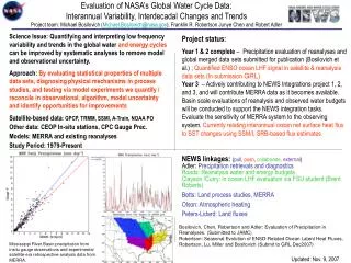
1. Evaluating the variability and budgets of global water cycle components V. Sridhar1, G. Goteti2, J. Sheffield2, J. Adam1 D.P. Lettenmaier1, E.F. Wood2 andC. Birkett3 1Department of Civil and Environmental Engineering Box 352700, University of Washington, Seattle, WA 98195 2 Princeton University, Princeton, NJ 3 NASA/GSFC, Greenbelt, MD

2. Global Water Cycle-Introduction • Thermohaline circulation of the world ocean is due to the flux of continental freshwater. • The surface water balance eqn.over land is dS/dt = P-E-Q Where P – Precipitation; E-Evapotranspiration; and Q is streamflow S is the sum of dominant terms ( soil moisture, snow water storage and lakes, wetlands and impoundments)

3. Global Water Cycle-Introduction(contd.) • The surface energy budget eqn. is Rn = LH+SH+GH Where Rn-Net radiation; LH-latent heat flux; SH-ground heat flux and GH- Ground heat flux • Changes in the water cycle due to natural variability and anthropogenic causes are linked as evaporation is common in both water and energy balance equations. • Therefore, understanding each term and its variability becomes important to get the budgets to balance.

4. Models considered in this study • Parallel Climate Model (PCM): • It is a coupled climate model that executes on the Cray T3E computer • The components are interfaced by a flux coupler that passes the energy, moisture, and momentum fluxes between components. • Under numerous forcing scenarios model runs have been made by NCAR and simulations have reprocessed by the PCMDI. Historic run B06.27 is used here. • Variable Infiltration Capacity (VIC) Atmospheric/landsurface component Ocean component Sea ice component

5. Hydrology Model -VIC • Multiple vegetation classes in each cell and are specified by their leaf area index, root distribution and canopy resistances • Sub-grid elevation band definition (for snow) • Snow pack accumulation and ablation simulated by a 2-layer energybalance model with canopy effects • 3 soil layers used • Explicit 2-layer parameterization for ground heat flux • Energy and water budget closure at each time step • Subgrid infiltration/runoff variability • Non-linear baseflow generation

6. Seasonal and Interannual variability • Quantification of variability in water budget components * MSV---the mean of the monthly range (maximum minus minimum) in the 21-year global simulations * MIAV---the mean absolute difference in annual totals for each of the variables

7. MSV-Preciptation • Both PCM and VIC model, show a predominent seasonal change in precipitation along the equatorial low (where precipitation is abundant in all seasons) • Subtropical high (North and southern Hemisphere) exhibit relatively moderate change (dry in all seasons). VIC PCM

8. MIAV-Precipitation • MIAV is quite distinct in the equatorial low (over Amazon basin) and mid-latitudes (of USA) and in South Asia. • Subpolar low regions (Alaska, Canada) shows some variability (where precipitation is abundant) • A high variability in the “source” term is expected to have strong impact on other water budget components. VIC PCM

9. MSV-Evaporation • MSV in Evaporation is quite high both in equatorial and subtropical high regions. • The only region that showed less changes are sub-Sahara Africa and Australian desert. • Evaporation variability is partly driven by variabilities in precipitation. VIC PCM

10. MIAV-Evaporation • MIAV is relatively less from VIC simulations across the continents, except Australia. • PCM displays higher variability over much of Africa, Australasia and S. America. VIC PCM

11. MSV-Change in SWQ • Greater change in snow water equivalent is obvious over high latitudes. • Obviously absense of snow in the lower regions and thereby no variabilities, except over Himalayas. VIC PCM

12. Higher MSV in precipitation (~270 mm) results in high variability in runoff (~50 mm) over S. America • Europe and S. America exhibit high variability (~80 mm) in evaporation that is equal in magnitude. • Out of Asia, Europe and N. America—more varibility in snow water equivalent is in N.America. • MSV in soil moisture is about 50-60 mm across all continents

13. The magnitudes of MIAV is relatively less than those of MSVs for all variables. • MIAV in precipitation is the highest for S.America followed by Australia and Europe and Asia show the least. • Australia hasthe highest MIAV in evaporation • Runoff variability is quite significant for S. America and Oceania that reflects the variability in precipitation as well. • Variability in snow water equivalent is the highest for N. America followed by Europe. • Australia has the highest variability in soil moisture and average is about 50 mm, equal in magnitude as that MSV.

14. Lakes, Wetlands and Impoundments • Lakes and wetlands are good indicators of climate change. They play a major part in global water budget computations. • Measurements of levels of lakes and wetlands are difficult and observations are sparsely available. • Remote sensing of lake and wetland levels becomes crucial. • A few major African lakes and wetlands data from TOPEX/POSEIDON satellite was made available to us by Charon Birkett, GSFC/NASA • They constitute 8.4 % of total lakes and 5% of the total land area.

15. Lake Level Changes Lake Area(km2) Lake Area(km2) Nyasa 6400 Turkana 6750 Tana 3600 Victoria 68800 Tanganyika 32000 Sudd Marshes ~10000

16. Mean seasonal change in lake level is about 275 mm (~14 mm for 5% of the total land area) Mean interannual change is about 2.3 mm. Exclusion of change in lake storage in the water budget equations is therefore expected to cause closure problems in surface water budget.

17. Conclusion • VIC showed a relatively low variability, but mostly in line with PCMs variability spatially. • Variabilities are high in S. America, Australia and Africa • Soil moisture did not include change in storage in wetlands, lakes and impoundments and that is expected to cause potential closure problems in surface water balance computations.

18. Land vs Atmospheric Water Budget • Atmosphere and land water budgets linked by P and E • Land atmosphere feedbacks: • climate variations, precipitation recycling, vegetation dynamics, … • Objectives of this study: • determine annual/seasonal atmospheric and land water budgets • NCEP/NCAR Reanalysis • VIC land surface simulations • determine where the 2 budgets differ • evaluate the NCEP/NCAR Reanalysis atmospheric moisture

19. Water Budget Equations D Atmosphere P E R Land On mean annual scales:

20. PrincetonUniversity Data NCEP/NCAR Reanalysis • 50+ years, 1948-present • Global coverage • T62 spectral resolution • Variables: • Assimilation of observations (surface, radiosonde, aircraft) • Model derived variables, e.g. precipitation, evaporation, runoff • Nudging  unclosed water budget VIC Land Surface Dataset • 50+ years, 1948-1998 • Global extra-polar land coverage • 2 degree • Forced with: • NCEP/NCAR Reanalysis near surface meteorology • NCEP/NCAR Reanalysis with near surface meteorology and corrected precipitation • Closed water budget

21. Atmospheric Budget: Reanalysis Annual 1950-1996 mean (mm) Evaporation (mm) Precipitation (mm) E-P (mm) Divergence (mm)

22. Land Budget: Reanalysis Annual 1950-1996 mean (mm) NCEP Evaporation (mm) NCEP Precipitation (mm) NCEP E-P (mm) NCEP Runoff (mm)

23. Land Budget: VIC forced by Reanalysis Annual 1950-1996 mean (mm) VIC Evaporation (mm) NCEP Precipitation (mm) VIC E-P (mm) VIC Runoff (mm)

24. Land Budget: VIC forced by corrected NCEP precipitation Annual 1950-1996 mean (mm) VIC Evaporation (mm) NCEP Corrected Precipitation (mm) VIC Runoff (mm) VIC E-P (mm)

25. Reanalysis Budget at Seasonal Scales Seasonal Mean 1950-1996 D – (E-P) (mm) (D – (E-P))/D (%) DJF DJF JJA JJA

26. Reanalysis Budget at Annual Scales Annual Mean 1950-1996 D – (E-P) (mm) (D – (E-P))/D (%)

27. D P E -R E-P Annual Land-Atmosphere Budget Land: NCEP/NCAR Reanalysis, Atmosphere: NCEP/NCAR Reanalysis Europe N. America Asia S. America Africa Oceania

28. D P E -R E-P Annual Land-Atmosphere Budget Land: VIC with NCEP meteorology, Atmosphere: NCEP/NCAR Reanalysis Europe N. America Asia S. America Africa Oceania

29. D P E -R E-P Annual Land-Atmosphere Budget Land: VIC with NCEP corrected meteorology, Atmosphere: NCEP/NCAR Reanalysis Europe N. America Asia S. America Africa Oceania

30. D P E -R E-P Examples of Budget Discrepancies Niger, NE Africa Amazon, S. America Ganges, S. Asia Mississippi, N. America Murray, Australia Lena, Russia

31. Worth of Reanalysis Data NCEP – NVAP (mm) (NCEP – NVAP)/NVAP (%) DJF DJF JJA JJA

32. Worth of Reanalysis Data Average Seasonal Vertically Integrated Moisture Content (mm) Africa DJF Asia DJF Europe DJF Africa JJA Asia JJA Europe JJA

33. Worth of Reanalysis Data Average Seasonal Vertically Integrated Moisture Content (mm) N. America DJF Oceania DJF S. America DJF N. America JJA Oceania JJA S. America JJA

34. Conclusions • Analyzed land and atmospheric water budgets for 1950-1996 using • NCEP/NCAR Reanalysis and • VIC forced with reanalysis • Known non-closure in reanalysis water budget shown • Generally higher variability in budget in S. America and Africa • D generally not consistent with E-P on annual scales especially in southern hemisphere • Reanalysis atmospheric moisture compares well with NVAP in Europe and N. America, but bias and scatter in southern hemisphere and Asia

35. Sources of Error • Use of average monthly q and (u,w) to calculate D • Comparison with NVAP • Monthly average values • Horizontal resolution (sharp gradients, steep topography) • Vertical resolution – pressure coordinates used (not model coordinates)

36. Observations used in Reanalysis Data Radiosonde Observations Jan 1991 Surface Observations Jan 1991 Aircraft Observations Jan 1991 CPC NCEP/NCAR Reanalysis Project web page http://wesley.wwb.noaa.gov/reanalysis.html

37. Annual Statistics Annual Mean 1950-1996 (mm) NCEP VICncep VICncep corrected Annual StdDev 1950-1996 (mm) NCEP VICncep VICncep corrected