Download
1 / 18
180 likes | 306 Vues
Time Dependent Estimates of the Velocity Gradient Tensor Field for Transient Detection. William Holt , Gina Shcherbenko, Eric Caruso, Yu Chen Acknowledgements: We thank SCEC for funding support. 0.1° x 0.1° Grid. Rigid Pacific Plate.

E N D
Time Dependent Estimates of the Velocity Gradient Tensor Field for Transient Detection William Holt, Gina Shcherbenko, Eric Caruso, Yu Chen Acknowledgements: We thank SCEC for funding support
0.1° x 0.1° Grid Rigid Pacific Plate
Model magnitude of shear strain rates (pure SS style)(SCEC4.0 Velocity field)
Smoothing or Damping • Maximize signal associated with GPS • Achieve Reduced Chi-Squared misfit between model displacement and observed displacement of ~1.0 for all epochs Haines, Jackson, Holt, Agnew [1998] Beavan and Haines [2001]
Time Series from SCEC IVc Red = 15 day moving average filter 4th order polynomial fit with annual and semi-annual terms Annual and semi-annual removed Green = 4th order polynomial WNRA – Phase 4c
Output 2 week epoch solutions of displacement Subtract out ‘master solution’ to estimate signal only from transients -For real data we used SCEC4.0 solution as a master solution -For other groups in the SCEC exercise we used time averaged solution (2007 – 2009). 5 mm 2 Week Displacements
Output 2 week epoch solutions of displacement Subtract out ‘master solution’ to estimate signal only from transients -For real data we used SCEC4.0 solution as a master solution -For other groups in the SCEC exercise we used time averaged solution (2007 – 2009). Phase IVa 5 mm 5 mm 2 Week Displacements Residual Displacements
What Triggers Selection of Potential Transients? • Accelerations • Finite Strain • Analysis of finite strain tensor and displacement vector fields • Does signal look tectonic?
Phase IVa Residual displacements reference solution subtracted out
Phase IVb Residual displacements reference solution subtracted out
Phase IVc Residual displacements reference solution subtracted out
Finite Displacements + Finite Strain (Principal Axes) Phase IVc
Summary of results from Phase IV • The modeling of displacements with reference field removed captures spatial and temporal magnitudes of transients • Method can be automated
Analysis of PBO Data from 2010.35 – 2011.25 • El Mayor-Cucapah post-seismic motions and strains • Non-steady state motions with periods of apparent increasing and decreasing strain • High frequency strain changes in LA Basin region
Finite Strain (Dilatations) + displacements: PBO Data 2010.35 – 2011.25 See poster B-143
Residual displacements show rapid spatially correlated changes in LA region 2010.35