Download

1 / 18
180 likes | 416 Vues
Monitoring Air Quality Changes Resulting from NO x Emission Regulations over the United States Using OMI and GOME-2 Data. Kenneth Pickering, NASA-Goddard Ana Prados, UMBC/JCET Edward Celarier, UMBC/GEST Robert Pinder, US EPA Shobha Kondragunta, NOAA/NESDIS. Introduction.

E N D
Monitoring Air Quality Changes Resulting from NOx Emission Regulations over the United States Using OMI and GOME-2 Data Kenneth Pickering, NASA-Goddard Ana Prados, UMBC/JCET Edward Celarier, UMBC/GEST Robert Pinder, US EPA Shobha Kondragunta, NOAA/NESDIS
Introduction • Tropospheric NO2 observations from space : GOME 8/95-6/03 40 x 320 km* 10:30 AM LT SCIAMACHY 8/03 60 x 30 km** 10:00 AM LT OMI 11/04 13 X 24 km*** 1:30 PM LT GOME-2 3/07 40 X 80 km 9:30 AM LT * Global coverage in 3 days; **complete coverage at Equator in 6 days; ***nadir resolution, increasing to 40 X 160 km at edges • Trend analyses – examples: Richter et al. (2005): GOME and SCIAMACHY data used to show NO2 increases over China and decreases in US and Europe Kim et al. (2006): SCIAMACHY data used to demonstrate initial NO2 decrease due to SIP Call power plant emission reduction
2-dimensional CCD wavelength ~ 780 pixels ~ 580 pixels viewing angle ± 57 deg flight direction » 7 km/sec 13 km (~2 sec flight)) 2600km 13 km x 24 km (binned & co-added) Aura/OMI Ozone Monitoring Instrument Aura Wavelength range: 270 – 500 nm Sun-synchronous polar orbit; Equator crossing at 1:30 PM LT 2600-km wide swath; horiz. res. 13 x 24 km at nadir Global coverage every day O3, NO2, SO2, HCHO, aerosol, BrO, OClO
GOME-2 on EUMETSAT/MetOp-A MetOp-A is the first of a sequence of three satellites to be launched at ~ 5-year intervals Wavelength range: 240-790 nm Sun-synchronous orbit with Equator crossing at 9:30 AM LT Near global coverage every day 80 x 40 km pixels Scan width: 1920 km NO2, BrO, SO2, HCHO, OClO, O3
What has happened to Eastern US NOx emissions since 2002? • US EPA mandated power plant NOx emission reductions under the 1998 NOxState Implementation Plan Call. Nearly 40% reductions between 2002 and 2005 were documented by Kim et al. (2006) using SCIAMACHY NO2 data. • Program has evolved into what is now called the “NOx Budget Trading Program”. Results in further summertime power plant emission reductions over the regulated region (19 eastern states) as a whole, but trading program allows flexibility concerning the magnitude of reduction at specific facilities. Over 2500 large combustion units affected. • Clean Air Interstate Rule (CAIR) – would have resulted in further reductions (28 states), but rule thrown out by courts; then reinstated; implementation procedures still being decided. Some companies reduced emissions in response to more stringent state rules and court orders.
Tier II Tailpipe NOx Emission Standards – 5% reduction in emissions per year for new vehicles over 2002 to 2010. Increasing Vehicle Miles Traveled largely negated the reductions until 2008. But, most recent national inventory including vehicle emissions is for 2005. US Monthly Vehicle Miles Traveled ~5% decr. Federal Highway Administration
Analysis Plan • Compute tropospheric NO2 trends from OMI for “regions of influence” around major clusters of power plants (e.g., Western PA, segments of Ohio Valley, etc.) defined by CMAQ output (2006 CONUS simulation including lightning NO emissions). In progress. • Region boundaries can be defined by looking for where power plant maxima in NO2 decays to near regional background levels subtracting CMAQ NO2 from run without power plant emissions from run with these emissions • Current analysis – focus on regional trends in Eastern and Central US and for 7 clusters of states.
July 2008 vs. July 2005 OMI Trop. NO2 -- % change Continuous Emission Monitoring System (CEMS) -- Absolute Changes
Extending the Trends Through 2009 Uncertainties on use of OMI Standard Product for trends in 2009: • Row anomaly become more significant in January 2009; lesser number of valid samples than in prior years • Change in albedo climatology (GOME OMI) in February 2009 Therefore, Summer 2009 was reprocessed using GOME albedo climatology for use in trend analysis Extended analysis to include MetOp-A/GOME-2 Trop. NO2 from NOAA/NESDIS: Slant columns – using Harvard algorithm, but with differences from KNMI minimized as much as possible Otherwise, all portions of tropospheric NO2 column algorithm are the same as for OMI Standard Product; GOME albedo climatology used. Morning overpass; 40 x 80 km pixels
July 2009-2008 PA: 0 to -20% IA, MO: +20 to +50% NY MD: 0 to -20% # of days
July 2009-2005 PA: -10 to +40% SD MO: +10 to +50% NYC-VA: -40 to -10% Chicago: -40 to -20% OH Valley: -25 to +25% June – less negative trends August – more negative trends
Extending the trends through 2009 For comparing means between years and instruments: Use statistic called the “standard deviation of the mean” = σ/N1/2 Too small to be visible on these plots! CEMS emission trend reversed from 2008 to 2009; OMI agrees only in July; GOME-2 agrees in June & July OMI PM obs. become closer to GOME-2 AM obs. going from June to August. NO2 loss rate becomes slower. OMI Albedo Clim
Generally, lower values of OMI NO2 when OMI albedo climo is used
OMI trends with use of OMI albedo climo. are in better agreement with CEMS. Would GOME-2 trends with OMI albedo climo also be in better agreement with CEMS? OMI Albedo
2008-2009 Trend Direction Comparisons OMI NO2 (with GOME albedos) CEMS 5/21 region-months in agreement OMI NO2 (with OMI albedos) CEMS 12/21 GOME-2 NO2 (with GOME albedos) CEMS 12/21 OMI NO2 (with GOME albedos) GOME-2 10/21 OMI NO2 (with OMI albedos) GOME-2 10/21
2005 – 2009 Trends Summary • Large summertime reductions in NO2 seen over much of eastern US over 2005 to 2008, except in the state of Pennsylvania. • After reprocessing with consistent surface albedo, some reversals of these trends are seen for 2008 to 2009 (e.g., Penna, Iowa). • Trends from 2008 to 2009 for regional monthly mean OMI NO2 retrieved using OMI albedos better agree with CEMS than those using GOME albedos. • Overall 2005 to 2009 summer trends remain strongly negative over much of the Eastern and Central US (with exceptions and with some regions having especially large downward trends).
Trends Summary • Monthly mean difference between GOME-2 and OMI tropospheric column values decreases from June August, reflecting slowing of NO2 daytime loss rate. • Disagreements between CEMS NOx emissions trends and satellite NO2 trends suggest that satellite instruments are “seeing” motor vehicle emissions perhaps better than has been thought. • Entire OMI NO2 period of record will be reprocessed using a new algorithm and consistent albedo climatology in the next year or so, allowing better trend assessment. • Loss of data due to row anomaly suggests that for trend analysis we should reprocess prior years using only the same pixel positions that were available for 2009.
The Future for NO2 Air Quality from Space • DISCOVER-AQ -- a NASA Earth Venture - 1 airborne and ground mission to improve understanding of the relationship between column gas and aerosol observations from space and surface air quality (J. Crawford, PI; K. Pickering, Project Scientist) Focus is on NO2, O3, and aerosols. Series of four field experiments. In-situ profiling, airborne remote sensing, surface-based remote sensing, surface in-situ air quality First experiment in Summer 2011 in Baltimore/Washington region. • GEO-CAPE -- NRC Decadal Survey Tier II mission – geostationary observations of trace gases and aerosols over North America. Hourly measurements at 4-km resolution. NO2, O3, HCHO, SO2, CO, aerosol Will lead to better understanding of emissions, transport and chemistry